21  Instruction Tuning and Preference Learning

Chapter tools Lecture slides 11.1 · ICL, Prompt Engineering, and RAG·Lecture slides 11.2 · Parameter-Efficient Fine-Tuning·Lecture slides 11.3 · Quantization and QLoRA·Download notebook·Open in Colab (opens in a new tab)

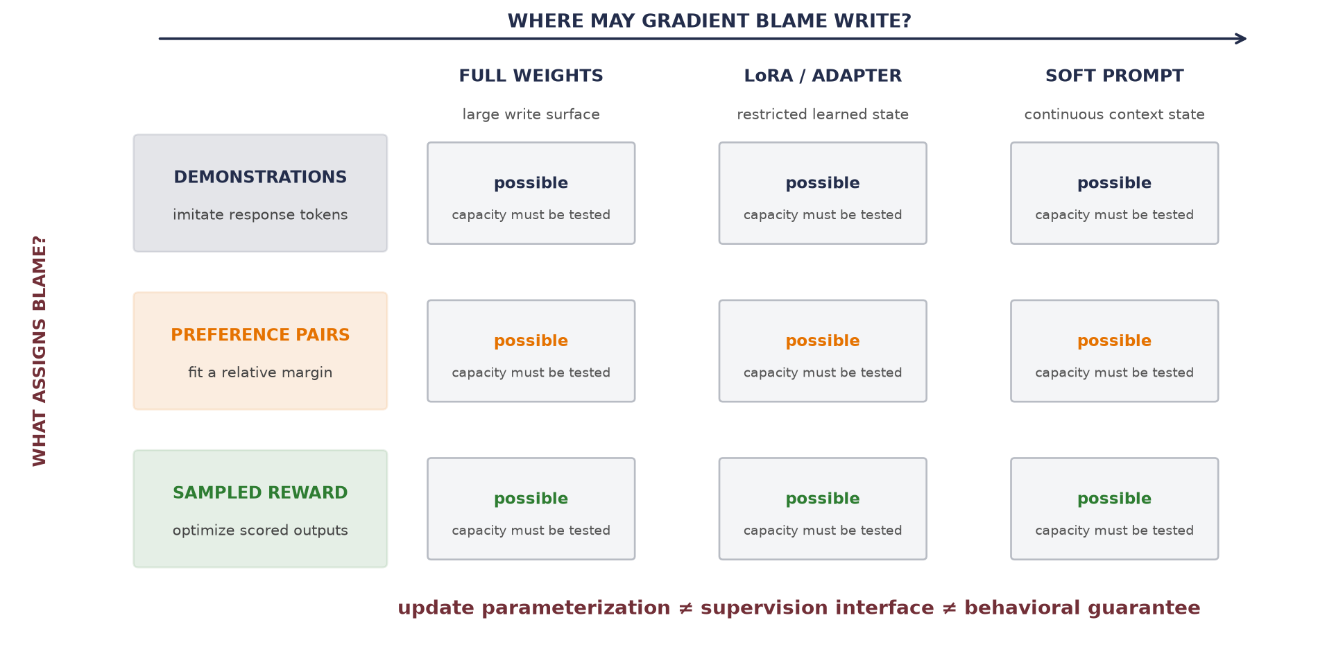
We saw in Chapter 20 that where the update lives is not what the update optimizes. Full fine-tuning, LoRA, and a soft prompt choose different places for the gradient to write. None of them says what should count as a good answer.

This chapter changes what the update optimizes. Pretraining asks for the next corpus token. Instruction tuning asks a model to imitate demonstrated responses. Preference learning asks which response wins a comparison. Online policy optimization asks a changing model to produce responses that score well under a reward signal. These supervision interfaces can often be paired with different update locations:

Figure 21.1: The objective and the update location are separate design axes. Demonstration loss, a preference margin, or sampled reward can supply the gradient while full weights, a low-rank branch, or continuous prompt vectors determine where that gradient may write. The grid marks possible combinations, not a claim that they have equal capacity or cost.

The word alignment is sometimes used as though it named one algorithm or one finished property; here it will mean something narrower and checkable: changing a model’s behavior toward a stated objective, for a stated prompt distribution and a stated population of evaluators. Helpful, honest, and harmless are useful names for the behavior we intend. They are not certificates that training can stamp onto a model.

The central problem is therefore a measurement problem. We need to specify whose judgment is collected, under which rubric, over which candidate responses, and what happens when optimization reaches beyond that coverage. Only then does it make sense to compare instruction tuning, reward-model pipelines, and direct preference optimization.

21.1 Same model, different supervision

Recall the causal language model from Chapter 16. Pretraining scores every corpus token that the model is asked to predict. In a prompt–response record, however, the prompt usually supplies the condition; the response supplies the supervised target. Let

\[ z=(x_1,\ldots,x_P,y_1,\ldots,y_T) \]

be a serialized prompt \(x\) followed by response \(y\). Define \(m_t=1\) when token \(z_t\) belongs to the response (including its end token) and \(m_t=0\) for prompt or padding positions. A response-masked supervised fine-tuning objective is

\[ \mathcal{L}_{\mathrm{SFT}}(\theta) =-\E_{(x,y)\sim\mathcal{D}_{\mathrm{demo}}} \left[ \frac{1}{\sum_t m_t} \sum_{t=2}^{P+T}m_t\log\pi_\theta(z_t\mid z_{<t}) \right]. \tag{21.1}\]

The displayed objective averages scored tokens within each response, then averages over prompt–response examples. Uniform sampling of examples gives a minibatch estimator of this per-example objective. Pooling all scored tokens within a batch instead gives longer responses more weight. The mask and both reductions must therefore be specified. The prompt is still essential because it conditions every response probability. Its tokens are simply not scored as targets in this version.

The tensor contract is explicit: logits has shape \((B,L,V)\), token IDs and the mask have shape \((B,L)\), and the returned sequence score has shape \((B,)\). The helper below checks that excluded prompt and padding targets cannot change that score.

1. Define the reusable completion_log_probability helper.
2. Score two masked toy sequences under random logits, then rescore after overwriting prompt and padding predictions.
3. Audit completion-only sequence log probabilities.

# [1]
def completion_log_probability(
    logits: Tensor, token_ids: Tensor, response_mask: Tensor
) -> Tensor:
    """Sum next-token log probabilities only at response positions."""
    if logits.shape[:2] != token_ids.shape or token_ids.shape != response_mask.shape:
        raise ValueError("logits, token IDs, and mask must share batch and time")
    next_token_logps = F.log_softmax(logits[:, :-1], dim=-1).gather(
        dim=-1, index=token_ids[:, 1:].unsqueeze(-1)
    ).squeeze(-1)
    return (next_token_logps * response_mask[:, 1:]).sum(dim=1)


# [2]
token_ids = torch.tensor([
    [1, 2, 3, 4, 5, 6, 0],
    [1, 2, 7, 8, 9, 6, 0],
])
response_mask = torch.tensor([
    [False, False, False, True, True, True, False],
    [False, False, True, True, True, True, False],
])
toy_logits = torch.randn(2, 7, 11)
original_logps = completion_log_probability(toy_logits, token_ids, response_mask)

perturbed_logits = toy_logits.clone()
inactive_predictors = ~response_mask[:, 1:]
perturbed_logits[:, :-1][inactive_predictors] = torch.linspace(-5, 5, 11)
perturbed_logps = completion_log_probability(
    perturbed_logits, token_ids, response_mask
)

# [3]
print("scored response tokens:", response_mask[:, 1:].sum(dim=1).tolist())
print(
    "largest change after perturbing prompt/padding predictions:",
    f"{(perturbed_logps - original_logps).abs().max().item():.2e}",
)

scored response tokens: [3, 4]
largest change after perturbing prompt/padding predictions: 0.00e+00

Instruction tuning is supervised fine-tuning on one or more tasks expressed through natural-language instructions. It changes the organization of the data, not the optimizer. FLAN, for example, studied whether instruction tuning across many tasks improved transfer to held-out tasks. That is an empirical result about its models and scale, not a theorem that every instruction dataset generalizes.

A useful shorthand says SFT teaches format while preferences teach quality, a distinction that is too sharp. A carefully written demonstration can teach facts, style, safety behavior, and substantive quality. Equation 21.1 says what SFT actually guarantees: it rewards probability assigned to demonstrated response tokens. It does not directly say why one unobserved response should be preferred to another.

Comparisons offer a different interface. For one prompt, a reviewer can sometimes choose between two candidates more reliably than they can write an ideal response from scratch. That generation–evaluation gap motivates preference data. It does not make comparison cheap in every domain, remove the need for expertise, or turn a judgment into universal truth.

Watch the mechanism: which predictor does the mask exclude?

Does the predictor at the last prompt slot contribute to the response score?

Word labels are illustrative aliases for the audit's unchanged token IDs, not tokenizer decoding. Every token wears its role, prompt or response; watch where the roles end up when the targets are built.

\( S_b=\sum_{i=0}^{5}\class{mp-mask}{m_{b,\class{mp-next}{i+1}}}\class{mp-logp}{\predictionpart{\log p_{b,i}(\targetpart{z_{b,\class{mp-next}{i+1}}})}} \)

Inputs stay available as context. Target masks select which log-probabilities enter the sum.

The mask and score receipt are readable without playback. Opening this panel loads the optional controls.

Here \(p_{b,i}\) is the model's next-token distribution given the entire prefix through slot \(i\), not just the word above it.

Scope and caveats

The supplied target at \(i+1\) selects a log-probability; its mask multiplies that score. The final padding input has no next target, so the aligned rows show six predictors and six shifted targets, including the padding target with ×0. This audit changes excluded output logits, not prompt input tokens, model parameters, or attention visibility. Changing the prompt could change the response probabilities. The helper returns a sequence sum of log probabilities; the SFT loss above negates and averages over scored response tokens. “Changed” is symbolic: no numerical probability or sequence score is claimed. The travelling copy and its one-slot slide are a drawing device for the helper's token_ids[:, 1:] and response_mask[:, 1:]: no tensor moves at run time, the role tags are the mask row spelt in words, and on a narrow screen each three-slot strip is a window on the same tape, so the copy that leaves the second strip by its left end is the one that enters the first strip on the right.

Check yourself. Suppose the response began at slot 1, so that slot 0 held the only prompt token. Would slot 0's prediction be scored?

Yes. Its target is the token at slot 1, the first response token, and the mask rides on the target: slid one slot left, that target lands under slot 0 with ×1. A scored predictor always sits one slot before its response target, so here the first one is at slot 0. Only a slot whose own next token is prompt or padding is excluded.

Transcript and keyboard help

1. Read sequence A using illustrative word aliases for the fixed IDs: prompt “Explain : why”, response “birds can fly”. Sequence B uses prompt “Explain :” and response “how planes also fly”. Each token card carries its own role tag, and each slot feeds one output. A marker rests under “why”, the last prompt slot. Predict whether that slot's output should count.
2. The targets are built in front of you. A copy of every token card, role tag attached, drops below the outputs; then the whole copy slides one slot to the left. “Explain” falls off the left end, the final “[PAD]” enters on the right, and “birds”, still tagged response, comes to rest under slot 2, whose input “why” is tagged prompt. The picture then holds still; nothing is gated yet.
3. Now the copies become the supplied targets. Each target's gate is read from the role tag that travelled with it: response gives ×1, prompt and padding give ×0. Row A scores targets “birds”, “can” and “fly” under slots 2, 3 and 4. The marker leaves “why”, takes slot 2's output along the side path to the gate of “birds”, passes ×1 and lands on the score rail. A predictor at slot \(i\) uses the whole prefix through that slot, not only the word above it.
4. Sequence B's response starts one slot earlier. Its copy makes the same one-slot slide, so “how”, tagged response, stops under slot 1: four targets are scored, under slots 1, 2, 3 and 4. The marker restarts at prompt slot 0, whose next target “:” is still a prompt token.
5. Hold sequence B fixed. Only outputs whose next targets have mask zero change, shown symbolically as “changed”. Both token sequences and all included terms stay fixed. A target's upward arrow selects its log-probability; the side path carries that score to the gate. An open gate's path runs on into the score rail; a closed gate's path ends at a stop bar.
6. The marker carrying slot 0's changed output stops at its ×0 gate and empties: each changed term is multiplied by zero. The audit prints zero change in either sequence score.
7. Revisit the boundary on sequence A: the marker runs from the last prompt predictor through the ×1 gate into the score, because the first response target has mask one.
8. The prompt remains context. Masking target loss does not remove input tokens or block attention.

Silent; paused initially; 1.5× playback. Focus the animation pane: Space or K plays/pauses, arrows seek between beats, Home/End jump, Escape pauses. The scrubber and speed menu also work by keyboard. Reduced-motion mode holds each beat's state instead of moving between them.

21.2 A preference is a measurement, not a value

One preference record contains a prompt \(x\), a response judged better \(y_w\), and a response judged worse \(y_l\):

\[ (x,y_w,y_l)\in\mathcal{D}_{\mathrm{pref}}. \]

The subscript \(w\) means winner under this comparison, not that the response is absolutely correct, harmless, or good. The label depends on the rubric, the reviewer population, the order in which candidates were displayed, and the policy that generated the candidates. Ties and disagreement are data, too; silently forcing them into a total order hides uncertainty.

To turn comparisons into a trainable scalar score, many pipelines use the Bradley–Terry model. A reward model \(r_\phi(x,y)\in\mathbb{R}\) assigns a score to each completed response. The probability of preferring one response depends on the score difference:

\[ P_\phi(y_w\succ y_l\mid x) =\sigma\!\left(r_\phi(x,y_w)-r_\phi(x,y_l)\right). \tag{21.2}\]

This is the sigmoid from Chapter 2. The corresponding negative log-likelihood is ordinary binary cross-entropy on a difference of scores:

\[ \mathcal{L}_{\mathrm{RM}}(\phi) =-\E_{(x,y_w,y_l)\sim\mathcal{D}_{\mathrm{pref}}} \log\sigma\!\left(r_\phi(x,y_w)-r_\phi(x,y_l)\right). \tag{21.3}\]

Only differences are identified. Adding any prompt-dependent constant \(c(x)\) to every candidate reward leaves Equation 21.2 unchanged. The model learns a ruler, one with no identifiable zero point.

There is a deeper assumption: all comparisons for one prompt must be representable by one scalar ordering. Let \(\vect{r}=(r_A,r_B,r_C)^\top\in\mathbb{R}^3\). Let the rows of \(\matr{B}\in\mathbb{R}^{3\times3}\) encode \(A-B\), \(B-C\), and \(C-A\). Then \(\matr{B}\vect{r}\) contains their three score differences. Bradley–Terry requires pairwise log-odds to be differences of the same scalar scores. Those log-odds must therefore sum to zero around every cycle. An acyclic preference ordering alone does not ensure this probability-level consistency. A cycle that prefers each response to the next cannot come from a score vector:

1. Fit least-squares scores to transitive and cyclic targets, then compute the scalar loss and its edgewise floor.
2. Make the scalar-reward assumption fail on a preference cycle.

# [1]
incidence = torch.tensor([
    [1.0, -1.0, 0.0],
    [0.0, 1.0, -1.0],
    [-1.0, 0.0, 1.0],
])

transitive_scores = torch.tensor([1.0, 0.0, -1.0])
transitive_targets = torch.sigmoid(incidence @ transitive_scores)
fitted_transitive = torch.linalg.lstsq(
    incidence, torch.logit(transitive_targets)
).solution
fitted_transitive -= fitted_transitive.mean()

cyclic_targets = torch.full((3,), 0.70)
fitted_cyclic = torch.linalg.lstsq(
    incidence, torch.logit(cyclic_targets)
).solution
fitted_cyclic -= fitted_cyclic.mean()
cyclic_predictions = torch.sigmoid(incidence @ fitted_cyclic)
scalar_loss = F.binary_cross_entropy(cyclic_predictions, cyclic_targets)
edgewise_floor = F.binary_cross_entropy(cyclic_targets, cyclic_targets)

# [2]
shifted_probabilities = torch.sigmoid(incidence @ (fitted_transitive + 37.0))
print("recovered centered scores:",   # + 0.0 prints a round-off -0.0 as 0.0
      [round(x, 6) + 0.0 for x in fitted_transitive.tolist()])
print("cyclic scalar predictions:", [round(x, 6) for x in cyclic_predictions.tolist()])
print(f"cyclic scalar loss: {scalar_loss.item():.6f}")
print(f"unconstrained edgewise floor: {edgewise_floor.item():.6f}")
print(f"irreducible scalar gap: {(scalar_loss - edgewise_floor).item():.6f}")
print(
    "largest probability change after adding 37 to every reward:",
    f"{(shifted_probabilities - transitive_targets).abs().max().item():.2e}",
)

recovered centered scores: [1.0, 0.0, -1.0]
cyclic scalar predictions: [0.5, 0.5, 0.5]
cyclic scalar loss: 0.693147
unconstrained edgewise floor: 0.610864
irreducible scalar gap: 0.082283
largest probability change after adding 37 to every reward: 0.00e+00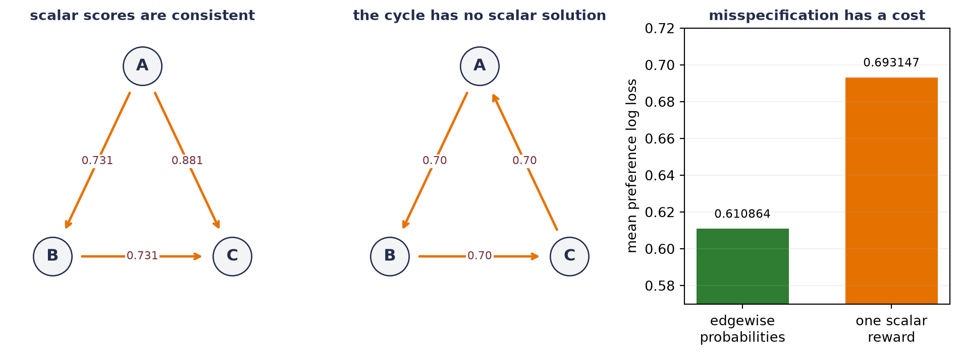

Figure 21.2: A scalar reward can express the transitive comparisons generated by centered scores (1, 0, -1), but not a symmetric cycle in which A beats B, B beats C, and C beats A with probability 0.70. Least squares returns equal scalar scores for the cycle, so Bradley–Terry predicts 0.50 on every edge. Its mean log loss is log 2 = 0.693147, above the unconstrained per-edge entropy 0.610864 by 0.082283.

The cycle is not a pathology in the code. Summing the three Bradley–Terry logits would require

\[ (r_A-r_B)+(r_B-r_C)+(r_C-r_A) =3\operatorname{logit}(0.70), \]

but the left side cancels to zero while the right side is positive. Aggregated human judgments can contain cycles because reviewers differ, context changes, or preferences are genuinely plural. A scalar reward model compresses that structure; it does not discover a hidden universal value.

WarningTrap: a preferred response is not scalar ground truth

A pair says which presented response won under one prompt, rubric, candidate set, and review process. Report ties and disagreement, split by prompt so that correlated pairs stay together, and state who supplied the judgments. Bradley–Terry is a useful model of those measurements, not proof that one population-independent reward exists.

Watch the mechanism: a preference ruler with no fixed zero

If every reward score increases by the same amount, does a response become more likely to win?

Follow responses A and C from the transitive example above. First read their score difference; then add the audit's common shift to both scores.

\( \predictionpart{P(A\succ C)}=\sigma\!\left(\class{pr-difference}{\predictionpart{r_A}-\predictionpart{r_C}}\right) \) \( =\sigma\!\left((\predictionpart{r_A}+\class{pr-cancel}{c})-(\predictionpart{r_C}+\class{pr-cancel}{c})\right) \)

Larger scores, same gap, same probability. The additions cancel: reward has no identifiable zero.

The calculation is readable without playback. Opening this panel loads the optional controls.

These are the existing transitive example's scores and common shift, not a new fit.

Scope and caveats

The viewport follows the scores while tick spacing stays fixed; it does not compress the gap. The Bradley–Terry probability models a comparison under one prompt and review process, not correctness or universal value. The constant may depend on the prompt but must be shared by its candidates. This invariance does not generally hold for unequal additions or rescaling. Cyclic judgments still need the separate audit above.

Check yourself. Instead of adding a constant, double both scores: 1 and −1 become 2 and −2. Does the preference probability change?

Yes. The gap doubles to 4 and the probability rises from 0.881 to 0.982. The model cannot see a common shift, but it does see a change of scale.

Transcript and keyboard help

1. Predict whether a common reward increase changes a pairwise preference probability.
2. The circle marks response A with score 1. The diamond marks response C with score minus 1.
3. The bracket measures A's score minus C's score: a gap of 2.
4. The sigmoid maps that gap to a modeled preference probability of approximately 0.881, the transitive figure's A-to-C edge.
5. Predict again before the shift: both scores will receive the same addition. Nothing moves during this beat; the ring records the probability before any motion.
6. One amount is added to both scores. After a still moment the pair slides as one, bracket and all, through half of the shift. The viewport follows with unchanged tick spacing, and the probability mark stays inside its ring.
7. Halfway, the gap is still 2 and the probability is still 0.881. The second half of the shift follows in the same way.
8. Adding 37 gives scores 38 and 36. Their gap is still 2 and their preference probability is unchanged: the two common additions cancel in the difference. Only relative scores are identified; a larger raw number is not a new measurement of goodness.

Silent; paused initially; 1.5× playback. Focus the animation pane: Space or K plays/pauses, arrows seek between beats, Home/End jump, Escape pauses. The scrubber and speed menu also work by keyboard. Reduced-motion mode holds each beat's state instead of moving between them.

21.3 Train a judge, then try to please the judge

What can we do with pairwise measurements? The classic language-model RLHF pipeline separates two learned objects:

1. a reward model learns to score completed responses from comparisons; and
2. a policy learns to generate responses that receive high score.

In one line: train a judge, then try to please the judge. The word judge matters. A reward model is a learned proxy for a feedback process, not the feedback process itself.

Figure 21.3: An original map of a reward-model RLHF pipeline. Demonstrations produce an SFT policy; sampled candidates and comparisons train a reward model. During online policy optimization, the current rollout policy produces responses, the frozen reward model scores them, and a fixed reference policy supplies a separate KL anchor. A value function estimates future shaped return from prefixes; it is not the reward model. PPO’s old-policy anchor is refreshed with rollout batches, while the reference anchor usually remains fixed.

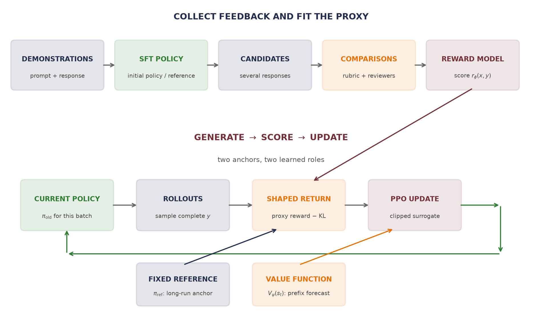
In language generation, the state \(s_t\) is the prompt plus tokens generated so far, the action \(a_t\) is the next token, and the policy is \(\pi_\theta(a_t\mid s_t)\). A reward model often scores the completed response. A separate value function \(V_\psi(s_t)\) estimates expected future shaped return from a prefix so that policy-gradient updates can assign credit across token decisions. Calling the reward model PPO’s critic conflates those two roles: completed-response scoring and prefix-value forecasting.

For a fixed prompt, suppose there are \(K\) complete candidate responses. Let \(\vect{r}\in\mathbb{R}^K\) contain their reward-model scores, and let \(\vect{\pi},\vect{\pi}_{\mathrm{ref}}\in\mathbb{R}^K\) be positive probability vectors that each sum to one. A KL-regularized objective is

\[ J(\vect{\pi}) =\sum_{i=1}^K\pi_i r_i -\beta D_{\mathrm{KL}} \!\left(\vect{\pi}\,\|\,\vect{\pi}_{\mathrm{ref}}\right), \qquad \beta>0, \tag{21.4}\]

where

\[ D_{\mathrm{KL}}(\vect{\pi}\,\|\,\vect{\pi}_{\mathrm{ref}}) =\sum_{i=1}^K\pi_i\log\frac{\pi_i}{\pi_{\mathrm{ref},i}}. \]

The first term seeks high proxy reward. The second charges for moving probability mass away from the reference. This is an objective to maximize, not a loss unless we negate it.

The exact finite-response policy

Before discussing an optimizer, we solve the finite problem. Add a Lagrange multiplier \(\lambda\) for \(\sum_i\pi_i=1\). Differentiating with respect to one probability gives

\[ r_i-\beta\left(\log\frac{\pi_i}{\pi_{\mathrm{ref},i}}+1\right)+\lambda=0. \]

Rearrange and absorb terms independent of \(i\) into a normalizer:

\[ \pi^*(y_i\mid x) =\frac{\pi_{\mathrm{ref}}(y_i\mid x) \exp\!\left(r(x,y_i)/\beta\right)} {Z(x)}, \qquad Z(x)=\sum_{j=1}^K\pi_{\mathrm{ref}}(y_j\mid x) \exp\!\left(r(x,y_j)/\beta\right). \tag{21.5}\]

Equation 21.5 is a reference distribution tilted toward higher reward. Large \(\beta\) resists movement; small \(\beta\) applies more reward pressure. In vector form the optimum is \(\vect{\pi}^*=\operatorname{softmax}(\vect{r}/\beta+\log\vect{\pi}_{\mathrm{ref}})\). This is the temperature softmax of Chapter 2 applied to the rewards, with \(\beta\) as the temperature and the reference log probabilities as fixed offsets that \(\beta\) does not scale. A large \(\beta\) shrinks \(\vect{r}/\beta\) toward zero, so the policy approaches \(\operatorname{softmax}(\log\vect{\pi}_{\mathrm{ref}})\), which equals \(\vect{\pi}_{\mathrm{ref}}\) because the reference already sums to one. Without the offsets, the same limit would be the uniform distribution. \(\beta\) controls drift, not truth or safety.

Consider four possible responses with

\[ \vect{\pi}_{\mathrm{ref}}=(0.55,0.25,0.15,0.05), \qquad \vect{r}=(0,1,2,3). \]

The reference favors response A while the proxy favors D. The exact solution lets us watch probability move without sampling noise or a language model:

1. Define the reusable helpers: gibbs_policy and kl_divergence.
2. Fix the four-response reference and reward, then tilt the reference at beta 4, 1, and 0.5.
3. Solve the KL-regularized finite-response policy exactly.

# [1]
def gibbs_policy(reference: Tensor, reward: Tensor, beta: float) -> Tensor:
    return torch.softmax(torch.log(reference) + reward / beta, dim=0)


def kl_divergence(policy: Tensor, reference: Tensor) -> Tensor:
    return (policy * (torch.log(policy) - torch.log(reference))).sum()


# [2]
reference = torch.tensor([0.55, 0.25, 0.15, 0.05])
reward = torch.tensor([0.0, 1.0, 2.0, 3.0])
shown_betas = [4.0, 1.0, 0.5]
shown_policies = [gibbs_policy(reference, reward, beta) for beta in shown_betas]

# [3]
sweep_betas = torch.logspace(math.log10(8.0), math.log10(0.2), 80)
sweep_policies = torch.stack([
    gibbs_policy(reference, reward, beta.item()) for beta in sweep_betas
])
sweep_rewards = sweep_policies @ reward
sweep_kls = torch.stack([
    kl_divergence(policy, reference) for policy in sweep_policies
])

target_policy = gibbs_policy(reference, reward, 1.0)
shifted_target = gibbs_policy(reference, reward + 37.0, 1.0)
print("beta  expected reward  KL to reference")
for beta in [4.0, 2.0, 1.0, 0.5, 0.25]:
    policy = gibbs_policy(reference, reward, beta)
    print(
        f"{beta:4.3g}      {(policy @ reward).item():.6f}"
        f"          {kl_divergence(policy, reference).item():.6f}"
    )
print("beta=1 policy:", [round(x, 6) for x in target_policy.tolist()])
print(
    "largest policy change after adding 37 to every reward:",
    f"{(shifted_target - target_policy).abs().max().item():.2e}",
)

beta  expected reward  KL to reference
   4      0.925670          0.029159
   2      1.191913          0.129706
   1      1.768029          0.561398
 0.5      2.559982          1.693801
0.25      2.944634          2.719127
beta=1 policy: [0.164562, 0.20333, 0.331625, 0.300483]
largest policy change after adding 37 to every reward: 8.33e-16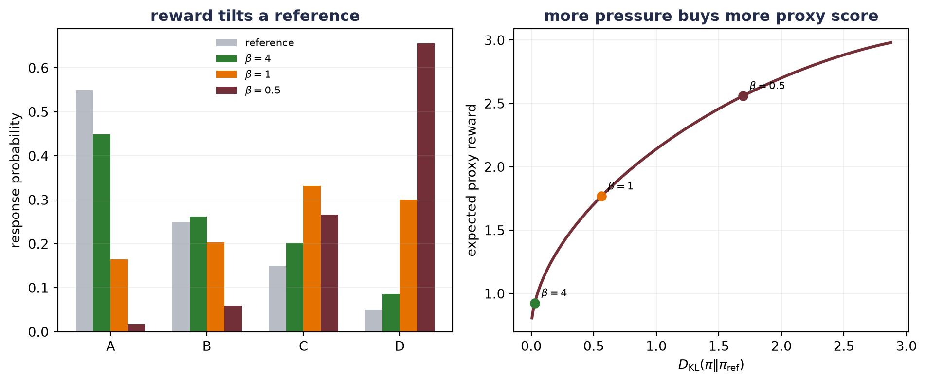

Figure 21.4: The exact four-response policy tilts the reference toward proxy reward. At beta 4, expected reward is 0.925670 and KL is 0.029159; at beta 1 they are 1.768029 and KL is 0.561398; at beta 0.5 they are 2.559982 and KL is 1.693801. Smaller beta raises proxy reward and measured drift together. This identity test assumes a complete finite response set and a correct scalar reward.

Watch the mechanism: what does more reward cost?

As the stay-near penalty weakens, what happens to proxy reward and drift from the reference?

The same four complete responses as the figure above. Gray outlines keep the reference visible; green bars show the exact policy at the current setting.

0.25 · more pressure4 · stays nearer

β =

0.50

\( \predictionpart{\pi_i^*}=\dfrac{\class{rt-reference}{\pi_{\mathrm{ref},i}}\,\class{rt-pressure}{e^{r_i/\beta}}}{\class{rt-normalizer}{\sum_j\pi_{\mathrm{ref},j}e^{r_j/\beta}}} \)

More proxy reward comes with more measured drift. Pressure does not repair the proxy.

The calculation is readable without playback. Opening this panel loads the optional controls.

This is the exact finite-response policy, not a training trajectory: the prompt, four candidates, positive reference and scalar proxy scores are fixed.

Scope and caveats

Smaller \(\beta\) increases expected proxy reward and measured KL here, but individual nonmaximal responses need not gain probability at every setting. Neither the score nor the stay-near dial establishes truth or safety. The slider changes an optimization setting, not a learned model parameter; probabilities are recomputed after subtracting the largest log-weight.

Check yourself. Push β toward zero. Where does the policy go, and how large can the KL from the reference become?

All of the probability moves to D, the response with the highest proxy score, and the KL approaches −ln 0.05 ≈ 2.996. Expected proxy reward tops out at 3. Nothing about the proxy has improved; the policy has only stopped listening to the reference.

Transcript and keyboard help

1. Predict. Gray outlines hold the reference probabilities for responses A through D. Fixed proxy scores are written beneath them, above two empty gauges. What will weakening the stay-near penalty change?
2. Start at the first printed setting. Green bars reveal the exact policy at beta four. These are already tilted probabilities, not the reference itself. Two gauges under the bars measure expected proxy reward and KL from the reference on fixed scales; a dashed mark on each shows where the reference itself sits.
3. Press harder. Beta falls toward one. Mass drains from A toward D, and both gauges lengthen together. All four probabilities come from the same normalized rule; the gray reference remains fixed.
4. Read the beta-one witness. The displayed probabilities and both readouts are computed from the unchanged fixture, agreeing with the audit above.
5. Press again. Beta falls toward one half. Response D gains more mass; a middle response can lose mass even though its score exceeds A's.
6. Read the beta-one-half witness. Proxy reward is higher, and so is KL drift. The policy remains a probability vector over exactly the same four candidates.
7. Audit the boundary. More pressure has purchased more proxy reward with more measured drift, not a guarantee of better answers. The single beta slider lets you inspect the same finite calculation.

Silent; paused initially; 1.5× playback. Focus the animation pane: Space or K plays/pauses, arrows seek between beats, Home/End jump, Escape pauses. The scrubber and speed menu also work by keyboard. The beta slider pauses playback and recomputes the picture; its arrow keys change beta, not time. Play or a timeline seek returns beta to the recorded sweep. The slider announces beta and both gauge values: three decimals while beta moves, the manuscript's six at the three witness holds. Reduced-motion mode holds each beat's state.

Adding 37 to every reward, as in the preference experiment, multiplies every unnormalized policy weight by the same \(e^{37/\beta}\), which changes \(Z(x)\) by that factor and leaves the normalized policy unchanged. Neither pairwise labels nor the regularized optimum identifies an absolute reward origin.

PPO in outline: a second anchor

Equation 21.5 optimizes directly over a finite probability vector. A language model instead has shared parameters, an enormous response space, and rewards that arrive mainly after a sequence is complete. Policy-gradient methods estimate how sampled token choices affected return. Proximal Policy Optimization (PPO) reuses a batch of trajectories while limiting the incentive to push each sampled action’s probability ratio outside a clipped interval.

For state \(s_t\), sampled action \(a_t\), current parameters \(\theta\), and the policy \(\pi_{\mathrm{old}}\) that generated the batch, define

\[ \rho_t(\theta) =\frac{\pi_\theta(a_t\mid s_t)} {\pi_{\mathrm{old}}(a_t\mid s_t)}. \]

If the advantage estimate \(\hat A_t\) indicates whether that sampled action did better or worse than the value baseline, PPO maximizes the clipped surrogate

\[ L^{\mathrm{CLIP}}(\theta) =\E_t\left[ \min\!\left( \rho_t(\theta)\hat A_t, \operatorname{clip}(\rho_t(\theta),1-\epsilon,1+\epsilon)\hat A_t \right) \right]. \tag{21.6}\]

This gives us two anchors, each with a different job:

• \(\pi_{\mathrm{old}}\) generated the current rollout batch. PPO refreshes it as training advances, and Equation 21.6 discourages the new policy from moving far from it on that batch.
• \(\pi_{\mathrm{ref}}\) is usually a fixed SFT policy. The KL term in Equation 21.4 addresses accumulated drift from that reference.

WarningThe old policy is not the reference policy

PPO clipping is not a hard wall on the new policy. It removes the favorable incentive for sampled ratios to move farther outside the interval. A large enough optimizer step can still overshoot, and unsampled behavior can still change. The fixed-reference KL discourages drift, but neither mechanism certifies retained capability or prevents proxy exploitation. Measure the realized KL and the behaviors that matter.

21.4 When the proxy becomes the target

The pipeline now has a vulnerable handoff: the reward model is validated on comparisons, but the policy is optimized to seek responses with high predicted reward. The compared responses and the responses the policy seeks come from different distributions. If the policy finds a region that the comparison data did not identify, excellent held-out reward-model loss can coexist with poor policy behavior.

NoteA designed mechanism study

Evidence and length are planted features. The finite candidate set is fully known; its designed utility is available because we wrote it. The study demonstrates how coverage failure and proxy pressure can interact. It does not estimate the prevalence of reward hacking in natural-language systems or validate one alignment method over another.

We can make that failure visible in a finite response world. Predict first: as reward pressure grows, will the designed utility of a policy optimized on narrow feedback rise, plateau, or rise and then collapse? Each synthetic response has two observable features:

• evidence \(e\), where larger means that more relevant support is present; and
• length \(\ell\), a stand-in for surface polish or detail.

The designed utility is

\[ u(e,\ell) =e+0.6\ell-1.2\max(\ell-1,0)^2. \tag{21.7}\]

Inside the feedback range \(0\le\ell\le1\), the curvature term is always zero. More detail helps there, so comparisons cannot reveal that excessive length should eventually become costly. We generate noisy Bradley–Terry comparisons per seed and fit the linear reward model

\[ \hat r(e,\ell) =w_e e+w_\ell\ell+w_q\max(\ell-1,0)^2. \]

We perform five complete runs with different seeds. A narrow-feedback arm sees only \(\ell\in[0,1]\). A coverage-repair arm draws 20% of individual comparison responses from \(\ell\in[1,4)\), where the missing curvature becomes observable. Both models have the same feature class and optimizer:

1. Define the reusable helpers: reward_features, designed_utility, and draw_responses.
2. Define the reusable helpers: fit_reward_model and mean_and_seed_sd.
3. List the five run seeds.
4. Fit five reward models with and without the missing feedback region.
5. Print weight means and seed SDs for both arms, then narrow and oracle in-range log loss and narrow order accuracy.

# [1]
def reward_features(responses: Tensor) -> Tensor:
    evidence = responses[:, 0]
    length = responses[:, 1]
    return torch.stack(
        (evidence, length, torch.relu(length - 1.0).square()), dim=1
    )


def designed_utility(responses: Tensor) -> Tensor:
    designed_weights = torch.tensor([1.0, 0.6, -1.2])
    return reward_features(responses) @ designed_weights


def draw_responses(
    count: int, generator: torch.Generator, out_of_range_fraction: float
) -> Tensor:
    evidence = torch.rand(count, generator=generator)
    length = torch.rand(count, generator=generator)
    if out_of_range_fraction > 0.0:
        outside = torch.rand(count, generator=generator) < out_of_range_fraction
        extended_length = 1.0 + 3.0 * torch.rand(count, generator=generator)
        length = torch.where(outside, extended_length, length)
    return torch.stack((evidence, length), dim=1)


# [2]
def fit_reward_model(
    seed: int, out_of_range_fraction: float
) -> tuple[Tensor, dict[str, float]]:
    generator = torch.Generator().manual_seed(seed)
    count = 20_000
    left = draw_responses(count, generator, out_of_range_fraction)
    right = draw_responses(count, generator, out_of_range_fraction)
    feature_differences = reward_features(left) - reward_features(right)
    preference_probabilities = torch.sigmoid(
        designed_utility(left) - designed_utility(right)
    )
    labels = torch.bernoulli(preference_probabilities, generator=generator)

    weights = nn.Parameter(torch.zeros(3))
    optimizer = torch.optim.Adam([weights], lr=0.05)
    for _ in range(900):
        logits = feature_differences @ weights
        loss = F.binary_cross_entropy_with_logits(logits, labels)
        optimizer.zero_grad()
        loss.backward()
        optimizer.step()

    held_left = draw_responses(10_000, generator, 0.0)
    held_right = draw_responses(10_000, generator, 0.0)
    held_differences = reward_features(held_left) - reward_features(held_right)
    held_probabilities = torch.sigmoid(
        designed_utility(held_left) - designed_utility(held_right)
    )
    held_labels = torch.bernoulli(held_probabilities, generator=generator)
    held_logits = held_differences @ weights.detach()
    held_nll = F.binary_cross_entropy_with_logits(held_logits, held_labels)
    oracle_nll = F.binary_cross_entropy(held_probabilities, held_labels)
    order_accuracy = (
        torch.sign(held_logits)
        == torch.sign(designed_utility(held_left) - designed_utility(held_right))
    ).double().mean()
    metrics = {
        "held_nll": held_nll.item(),
        "oracle_nll": oracle_nll.item(),
        "order_accuracy": order_accuracy.item(),
    }
    return weights.detach(), metrics


# [3]
seeds = list(range(6050, 6055))
# [4]
narrow_fits = [fit_reward_model(seed, 0.0) for seed in seeds]
repaired_fits = [fit_reward_model(seed, 0.20) for seed in seeds]
narrow_weights = torch.stack([fit[0] for fit in narrow_fits])
repaired_weights = torch.stack([fit[0] for fit in repaired_fits])

def mean_and_seed_sd(values: Tensor) -> tuple[Tensor, Tensor]:
    return values.mean(dim=0), values.std(dim=0, unbiased=True)

narrow_mean, narrow_sd = mean_and_seed_sd(narrow_weights)
repaired_mean, repaired_sd = mean_and_seed_sd(repaired_weights)
narrow_nlls = torch.tensor([fit[1]["held_nll"] for fit in narrow_fits])
oracle_nlls = torch.tensor([fit[1]["oracle_nll"] for fit in narrow_fits])
narrow_accuracies = torch.tensor([
    fit[1]["order_accuracy"] for fit in narrow_fits
])

# [5]
print("feedback               w_e       w_length   w_curve")
print("narrow mean       ", "  ".join(f"{x:.6f}" for x in narrow_mean))
print("narrow seed sd    ", "  ".join(f"{x:.6f}" for x in narrow_sd))
print("repaired mean     ", "  ".join(f"{x:.6f}" for x in repaired_mean))
print("repaired seed sd  ", "  ".join(f"{x:.6f}" for x in repaired_sd))
print(
    "narrow in-range NLL:",
    f"{narrow_nlls.mean().item():.6f} +/- {narrow_nlls.std(unbiased=True).item():.6f}",
)
print(
    "oracle in-range NLL:",
    f"{oracle_nlls.mean().item():.6f} +/- {oracle_nlls.std(unbiased=True).item():.6f}",
)
print(
    "narrow designed-order accuracy:",
    f"{narrow_accuracies.mean().item():.6f} +/- "
    f"{narrow_accuracies.std(unbiased=True).item():.6f}",
)

feedback               w_e       w_length   w_curve
narrow mean        1.004469  0.634378  0.000000
narrow seed sd     0.042489  0.019772  0.000000
repaired mean      0.984938  0.600285  -1.208128
repaired seed sd   0.073378  0.007907  0.025924
narrow in-range NLL: 0.665633 +/- 0.002097
oracle in-range NLL: 0.665603 +/- 0.002092
narrow designed-order accuracy: 0.992940 +/- 0.002548

The narrow model looks excellent where it was tested: its mean held-out log loss is 0.665633, only 0.000030 above the oracle that generated the labels, and its latent ordering accuracy is 0.992940. The coefficient \(w_q\) remains exactly zero: that feature was zero in every narrow comparison, so no gradient could identify its coefficient. A validation split drawn from the same support cannot expose the missing behavior.

Now place 401 candidate responses at fixed evidence \(e=0.72\) and lengths from zero to four. The reference policy is a discretized bell-shaped distribution with mean length 0.776439. For each fitted reward model and each \(\beta\), compute the exact policy from Equation 21.5. No sampled-policy optimizer is needed; any failure comes from the proxy and its feedback coverage:

1. Place 401 candidates at evidence 0.72 and lengths 0 to 4, and set a bell-shaped reference and four beta values.
2. Define the reusable policy_metrics helper.
3. Optimize the proxy outside its comparison coverage.

# [1]
lengths = torch.linspace(0.0, 4.0, 401)
evidence = torch.full_like(lengths, 0.72)
candidates = torch.stack((evidence, lengths), dim=1)
candidate_features = reward_features(candidates)
candidate_designed_utility = designed_utility(candidates)
reference_policy = torch.softmax(
    -0.5 * ((lengths - 0.695) / 0.5).square(), dim=0
)
pressure_betas = [1.0, 0.5, 0.25, 0.125]

# [2]
def policy_metrics(weights_by_seed: Tensor) -> dict[float, Tensor]:
    rows: dict[float, Tensor] = {}
    for beta in pressure_betas:
        seed_rows = []
        for weights in weights_by_seed:
            proxy = candidate_features @ weights
            policy = torch.softmax(
                torch.log(reference_policy) + proxy / beta, dim=0
            )
            seed_rows.append(torch.stack((
                policy @ lengths,
                policy @ proxy,
                policy @ candidate_designed_utility,
                kl_divergence(policy, reference_policy),
            )))
        rows[beta] = torch.stack(seed_rows)
    return rows


narrow_rows = policy_metrics(narrow_weights)
repaired_rows = policy_metrics(repaired_weights)
reference_length = reference_policy @ lengths
reference_designed_utility = reference_policy @ candidate_designed_utility

# [3]
print(f"reference mean length: {reference_length.item():.6f}")
print(f"reference designed utility: {reference_designed_utility.item():.6f}")
print("narrow feedback: beta  length  proxy  designed  KL")
for beta, values in narrow_rows.items():
    mean, seed_sd = mean_and_seed_sd(values)
    print(
        f"{beta:5.3f}  {mean[0].item():.6f}  {mean[1].item():.6f}"
        f"  {mean[2].item():.6f}  {mean[3].item():.6f}"
        f"  (designed sd {seed_sd[2].item():.6f})"
    )
print("repaired feedback: beta  length  proxy  designed  KL")
for beta, values in repaired_rows.items():
    mean, seed_sd = mean_and_seed_sd(values)
    print(
        f"{beta:5.3f}  {mean[0].item():.6f}  {mean[1].item():.6f}"
        f"  {mean[2].item():.6f}  {mean[3].item():.6f}"
        f"  (designed sd {seed_sd[2].item():.6f})"
    )

reference mean length: 0.776439
reference designed utility: 1.130480
narrow feedback: beta  length  proxy  designed  KL
1.000  0.901311  1.295055  1.164883  0.040327  (designed sd 0.000874)
0.500  1.037928  1.381796  1.183447  0.170991  (designed sd 0.000480)
0.250  1.335088  1.570472  1.135363  0.739579  (designed sd 0.007630)
0.125  1.963796  1.969632  0.484541  3.138049  (designed sd 0.067970)
repaired feedback: beta  length  proxy  designed  KL
1.000  0.837956  1.157585  1.168536  0.018632  (designed sd 0.000484)
0.500  0.895553  1.190942  1.201869  0.068282  (designed sd 0.000905)
0.250  0.990698  1.243968  1.254875  0.224387  (designed sd 0.001374)
0.125  1.104397  1.305569  1.316470  0.577948  (designed sd 0.001310)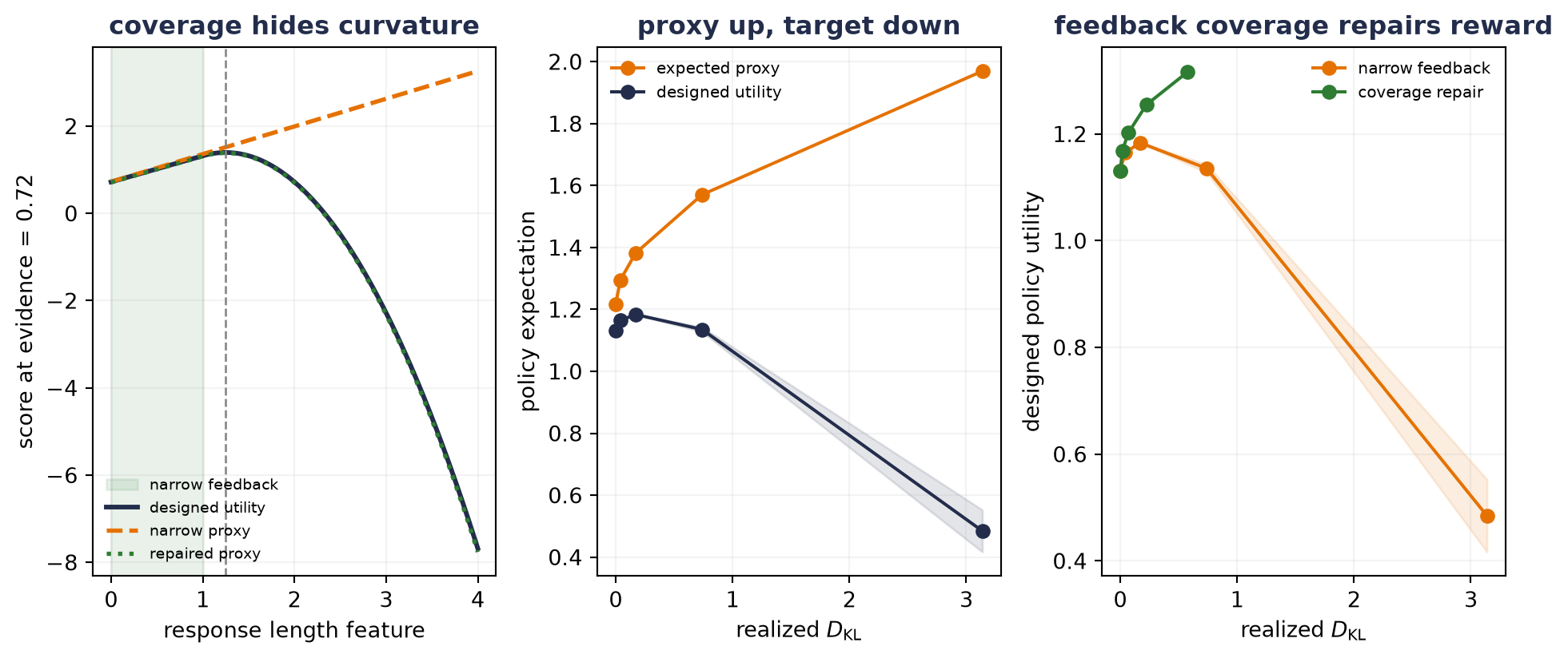

Figure 21.5: A reward model can pass an in-range comparison test and fail under optimization. Narrow feedback covers only the shaded length interval, so the learned proxy remains linear after designed utility turns down (left). Under increasing reward pressure, its expected proxy score rises while designed utility is highest among the four tested settings at beta 0.5 and falls to 0.484541 at beta 0.125, with realized KL 3.138049 (center). Adding 20% out-of-range responses identifies the missing curvature; at beta 0.125 the repaired policies retain mean designed utility 1.316470 (right). Lines are means over five reward-model seeds; designed-utility bands show one seed SD where plotted.

At moderate pressure, the narrow proxy helps: mean designed utility rises from 1.130480 under the reference to 1.183447 at \(\beta=0.5\). More pressure then reverses the result. At \(\beta=0.125\), mean predicted reward has climbed to 1.969632 while designed utility has fallen to 0.484541. The KL penalty changes how quickly the policy reaches the failure; it cannot invent the missing curvature.

The repair changes feedback coverage, not the policy optimizer; once 20% of individual responses expose the longer regime, the mean fitted curvature coefficient is \(-1.208128\) (designed value \(-1.2\)). At \(\beta=0.125\), the repaired policies reach mean designed utility 1.316470 instead of 0.484541. In this controlled world, better feedback coverage matters more than choosing a fancier route to the same proxy.

WarningReward-model validation is not policy validation

Held-out pair loss tests interpolation over a declared comparison distribution; policy optimization deliberately changes the response distribution. Evaluate current-policy outputs with independent judgments, track realized drift and length or style shifts, and refresh feedback where the policy now visits. A proxy score rising by itself is not evidence that the intended behavior improved.

21.5 DPO removes a stage, not the assumptions

Reward-model RLHF fits an explicit proxy, freezes it, then optimizes a policy against it. Can we use preference pairs without that separately trained middle model? DPO solves the optimal-policy relation, Equation 21.5, for the reward, then substitutes that reward into the preference model.

Figure 21.6: Two routes can consume preference pairs. A reward-model route first fits an explicit scalar proxy, then scores fresh outputs during online policy optimization. DPO forms a reference-adjusted policy margin directly on a fixed pair dataset. It removes the explicit reward-model stage and online sampling during the optimization pass, but both routes still depend on the preference rubric, coverage, a scalar-reward model, and an adequate reference support.

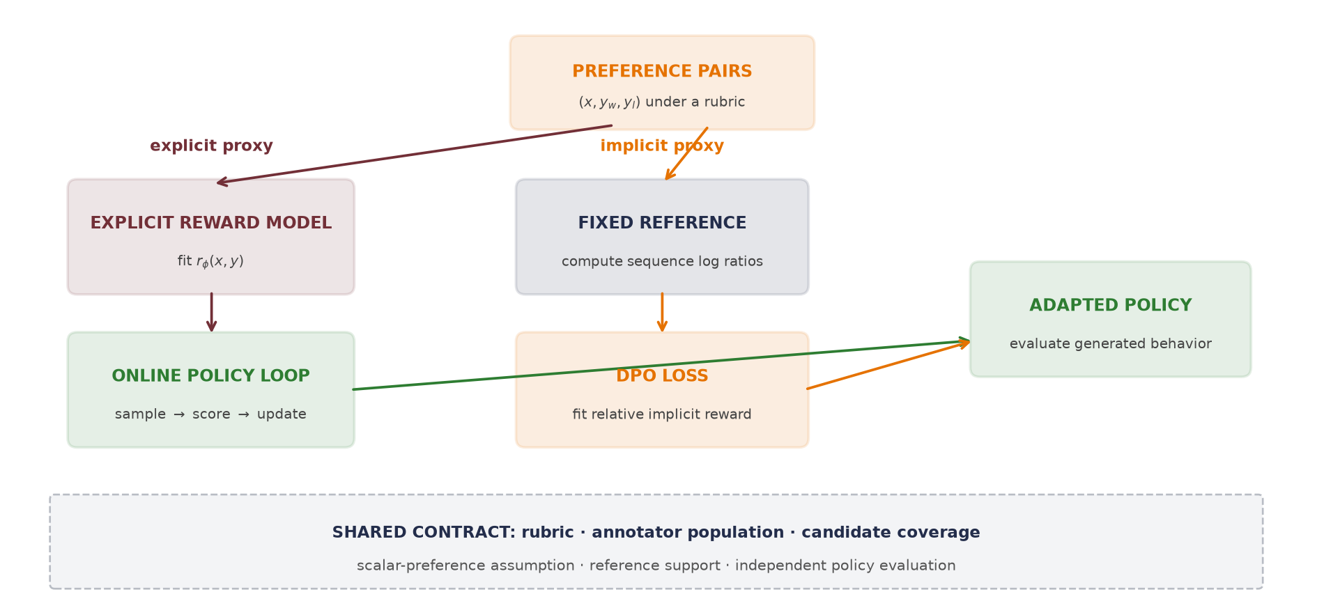
Rearrange the exact optimum:

\[ r(x,y) =\beta\log\frac{\pi^*(y\mid x)}{\pi_{\mathrm{ref}}(y\mid x)} +\beta\log Z(x). \tag{21.8}\]

For two responses to the same prompt, the \(\beta\log Z(x)\) term is identical and cancels from the reward difference. Define the current policy’s reference-adjusted score

\[ s_\theta(x,y) =\log\pi_\theta(y\mid x)-\log\pi_{\mathrm{ref}}(y\mid x). \]

Substituting Equation 21.8 into Bradley–Terry gives Direct Preference Optimization (DPO):

\[ \mathcal{L}_{\mathrm{DPO}}(\theta) =-\E_{(x,y_w,y_l)\sim\mathcal{D}_{\mathrm{pref}}} \log\sigma\!\left( \beta\left[s_\theta(x,y_w)-s_\theta(x,y_l)\right] \right). \tag{21.9}\]

For an autoregressive model, \(\log\pi_\theta(y\mid x)\) is a sum over response token log probabilities, normally including the response end token:

\[ \log\pi_\theta(y\mid x) =\sum_{t=1}^{T}\log\pi_\theta(y_t\mid x,y_{<t}). \]

The completion mask audited near Equation 21.1 applies here as well. Prompt and padding targets contribute zero; length-normalizing that sum would define a different objective and should be named as such.

Does the algebra work in the finite world? Use all six response pairs, but train on their exact stochastic Bradley–Terry probabilities rather than separable hard winners. For this identity check, set \(\beta=1\). The DPO logit for pair \((i,j)\) is \(\beta(s_i-s_j)\). Starting from the reference, optimize four unconstrained reference-relative offsets, identifiable only up to a shared additive constant:

1. Compute the six pair probabilities and analytic policy, then train four reference-relative offsets on the DPO loss.
2. Recover the exact regularized policy with DPO.

# [1]
pairs = torch.tensor([
    [0, 1], [0, 2], [0, 3], [1, 2], [1, 3], [2, 3]
])
dpo_beta = 1.0
pair_probabilities = torch.sigmoid(
    reward[pairs[:, 0]] - reward[pairs[:, 1]]
)
target_policy = gibbs_policy(reference, reward, dpo_beta)

log_ratio = nn.Parameter(torch.zeros(4))
dpo_optimizer = torch.optim.Adam([log_ratio], lr=0.05)
for _ in range(4000):
    comparison_logits = dpo_beta * (
        log_ratio[pairs[:, 0]] - log_ratio[pairs[:, 1]]
    )
    dpo_loss = F.binary_cross_entropy_with_logits(
        comparison_logits, pair_probabilities
    )
    dpo_optimizer.zero_grad()
    dpo_loss.backward()
    dpo_optimizer.step()

dpo_policy = torch.softmax(
    torch.log(reference) + log_ratio.detach(), dim=0
)
# [2]
print("analytic policy:", [round(x, 6) for x in target_policy.tolist()])
print("DPO policy:     ", [round(x, 6) for x in dpo_policy.tolist()])
print(
    "largest policy difference:",
    f"{(dpo_policy - target_policy).abs().max().item():.2e}",
)

analytic policy: [0.164562, 0.20333, 0.331625, 0.300483]
DPO policy:      [0.164562, 0.20333, 0.331625, 0.300483]
largest policy difference: 5.55e-17

The match to floating-point tolerance holds under deliberately strong conditions: a fixed positive reference, a complete finite response set, all pairwise comparisons, preferences generated by one scalar reward, adequate policy capacity, and successful optimization. It does not show that natural-language DPO and PPO are universally equivalent.

Several details are easy to overstate:

• DPO avoids an explicit standalone reward model and an online rollout loop during the optimization pass. Its policy–reference log ratio is still an implicit reward representation, and candidate generation plus labeling happened upstream.
• The reference need not be the exact behavior policy that generated every pair. It anchors the density ratio, so its support matters and choosing it is a modeling decision.
• \(\beta\) appears in the regularized derivation, but finite-data DPO does not enforce a hard realized-KL budget. Measure the KL.
• The gradient rewards a relative reference-adjusted margin. Shared parameters mean one optimizer step need not raise the winner’s absolute probability and lower the loser’s absolute probability separately.
• Offline pairs cannot correct missing candidate coverage by themselves. DPO can fit a stale or narrow preference dataset efficiently.

NoteWhat the finite identity proves

The four-response test validates the derivation inside its scalar-preference, support, coverage, capacity, and optimization assumptions. The cyclic and proxy-pressure audits test two ways those assumptions fail.

21.6 Choose by the feedback and exploration you have

There is no universal method ranking. Start by naming the information source and whether new responses must be explored during optimization, as Table 21.1 makes explicit:

Table 21.1: Feedback source and exploration needs determine which alignment route is available.

Route	Supervision	Fitted quantity	Fresh samples?	Main risk
Response-masked SFT	Demonstrated responses	Likelihood of demonstration tokens	No	Demonstration coverage and imitation target
DPO	Fixed preferred/rejected pairs	Reference-adjusted preference margin	No	Pair coverage, reference, scalar-preference assumptions
Explicit RM + online policy optimization	Comparisons plus a reward model; current responses can be scored	Reward proxy, value function, and policy objective	Yes	Proxy shift, exploration, credit assignment, optimization stability
Programmatic check + online policy optimization	Tests or exact answers applied to current responses	Value function and policy objective, with no reward model	Yes	Checker coverage, reward hacking

SFT may be enough when demonstrations directly specify the desired behavior. Fixed preference data may favor an offline direct method when comparison coverage is already good. Online methods can generate from the changing policy and request or compute fresh feedback, which matters when exploration is part of the task. They also have more ways to fail and more to evaluate.

When a program can check a response, as in the last row of Table 21.1, the judge need not be learned. Unit tests for generated code, or a match against the known final answer of a math problem, can set \(r_i=1\) when response \(i\) passes and \(r_i=0\) when it fails. The first term of Equation 21.4 then becomes the expected pass rate.¹ A checker has no fitting error, but it is still a proxy for the intended behavior. Generated code that handles only the tested inputs passes weak tests and earns full reward. Reward pressure can move the policy toward such responses, as it moved the narrow-feedback policies beyond the feedback range. Such a move is called reward hacking: the proxy score rises while the intended behavior does not improve.

The update location studied in Chapter 20 is a separate choice. SFT, DPO, or an online policy objective may update full weights, a LoRA branch, or another permitted state. Parameter efficiency changes the write surface and resource cost, not the rubric, comparison coverage, or reward fidelity.

Variants rearrange sampling, scoring, and labeling. Rejection-sampling fine-tuning selects high-scoring samples and imitates them. AI feedback replaces or supplements human labels but inherits the evaluator model’s coverage and biases. Constitutional AI, for example, combines supervised critique and revision with later preference-based RL guided by written principles.

21.7 Alignment is evaluated through a chain of evidence

An optimization loss is only one piece of the evidence; a report should connect the people and prompts that created feedback to independent tests of the policy that will actually be used:

Figure 21.7: Alignment evaluation is a chain of evidence, not one score. The feedback record identifies the rubric, reviewers, prompts, candidates, ties, and disagreement. Reward-model audits hold out prompts and test calibration and newer-policy responses. Policy audits add blinded judgments, realized KL, length and style shifts, retained capabilities, and relevant slices. A model card records intended and out-of-scope uses, data and feedback provenance, limitations, and versioning; it does not certify safety.

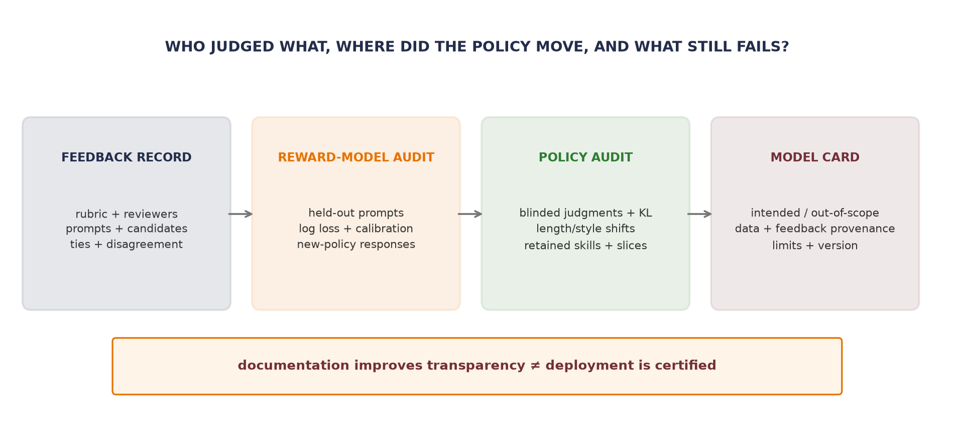
The feedback report should identify the prompt distribution, selection policy for candidates, rubric, reviewer population, and aggregation rule. If several pairs came from one ranked set, they are correlated; keep pairs from the same prompt in the same split and cluster uncertainty at the prompt level. Randomize A/B order, retain ties, and disclose disagreement rather than converting it silently into certainty.

Reward-model evaluation should include held-out pair log loss, calibration or Brier score, and tests on candidates from newer policies. Policy evaluation must go beyond reward: blinded independent preferences, task-specific success, realized KL to the reference, response-length and refusal shifts, retained capabilities, and safety or domain slices relevant to intended use. Give sample counts and uncertainty. A raw gap between two slices is not automatically statistically meaningful.

An LLM can assist as a judge, another measurement instrument. Published audits have found position, verbosity, and self-enhancement biases. Blinding model identities, swapping candidate order, keeping ties, and validating against human judgments are important safeguards.

A model card is a nutritional label for a model. It records model and training details, intended users and uses, out-of-scope uses, data and feedback provenance, evaluation conditions, slice results, limitations, version, and contact. A label helps a reader make an informed decision; it does not prevent misuse, prove that omitted groups are safe, or convert a conditional evaluation into a certificate.

WarningTrap: alignment is not the whole ethics of a system

This chapter asks whether a model’s behavior meets a declared feedback rubric and holds up under a declared evaluation. That question matters, but it does not absorb every sociotechnical question around the system:

• Data and rights: privacy, consent, ownership, and the legitimacy of collection.
• Distribution of effects: who receives benefits, errors, exclusions, or recourse.
• Production: human labor, resource use, environmental cost, and supply chains.
• Governance and use: misuse, institutional incentives, accountability, oversight, and appeal.

A model card can expose these choices. It cannot confer consent, resolve values, assign accountability, or certify deployment. Appendix E states the limits of statistical evidence; ethical and governance judgment remains separate.

TipDeclare the evaluation before optimizing

Predeclare the rubric, feedback population, prompt and candidate coverage, ties, primary policy outcomes, retained capabilities, slices, decoding settings, and drift measure. Then a rising training objective has a declared external test. Without that test, “better aligned” can collapse into “the optimizer increased its own score.”

21.8 The next question: where did the generator come from?

A judge is not a generator: a reward model can rank or score completed responses; it does not explain how a model learned a distribution from which responses can be sampled. RLHF and DPO begin with a generator already in hand.

The autoencoder interlude already traced reconstruction from PCA’s linear geometry to trainable nonlinear codes. Chapter 22 asks how a model defines or learns a distribution and turns it into samples, then develops variational autoencoders, adversarial learning, and diffusion. Chapter 21 changes the behavior of a generator; Chapter 22 studies the machinery that makes generation possible.

NoteCheck yourself

Close the book for one minute and separate update location from objective.

• Which tokens contribute to the supervised fine-tuning loss?
• What information does a preference pair add beyond one demonstration?
• How do reward modeling, RLHF, and DPO differ in where the learned signal enters?

21.9 Okay, so: where to update and what to optimize are separate

1. Update location and objective are separate axes. Full tuning, LoRA, and soft prompts decide where gradients may write. SFT, preference margins, and sampled rewards decide what those gradients optimize.
2. SFT imitates demonstrated response tokens. A completion mask keeps prompt and padding targets out of the loss. Demonstrations can encode quality; preference data supplies a different, comparative signal.
3. A preference is conditional evidence. Bradley–Terry turns score differences into probabilities, but reward zero points are unidentified and cyclic aggregate preferences cannot fit one scalar ordering.
4. RLHF separates judge from actor. The reward model scores completed responses, the value function forecasts shaped return from prefixes, PPO uses a refreshed old policy, and reference KL uses a usually fixed anchor.
5. Reference KL is a pressure dial. The finite optimum is \(\pi^*\propto\pi_{\mathrm{ref}}e^{r/\beta}\). More pressure can raise proxy reward; it cannot repair a proxy’s missing feature.
6. DPO removes an explicit stage, not the assumptions. The four-response identity is exact under scalar preferences, compatible support, complete coverage, adequate capacity, and successful optimization. Realized KL and generated behavior still need measurement.
7. Alignment is evaluated, not certified. State who judged which candidates under what rubric, then evaluate the current policy independently and document intended use, slices, uncertainty, and limitations. This evaluation is one part of a broader ethical and governance assessment, not a substitute for it.

Sources and further reading

• Wei et al., Finetuned Language Models Are Zero-Shot Learners.
• Christiano et al., Deep Reinforcement Learning from Human Preferences.
• Stiennon et al., Learning to Summarize with Human Feedback: feedback training and overoptimization.
• Askell et al., A General Language Assistant as a Laboratory for Alignment: helpful, honest, and harmless framing.
• Ouyang et al., Training Language Models to Follow Instructions with Human Feedback: SFT, reward modeling, PPO, and scope.
• Schulman et al., Proximal Policy Optimization Algorithms: the clipped policy-ratio surrogate.
• Rafailov et al., Direct Preference Optimization: the reward–policy identity and DPO loss.
• Gao et al., Scaling Laws for Reward Model Overoptimization: controlled proxy-overoptimization studies.
• Mitchell et al., Model Cards for Model Reporting: documenting evaluation and intended use.
• Selbst et al., Fairness and Abstraction in Sociotechnical Systems: why a technical model must be read inside the social system where it operates.
• Raji et al., Closing the AI Accountability Gap: an end-to-end framework for internal algorithmic auditing.
• Zheng et al., Judging LLM-as-a-Judge: model-judge biases.
• Bai et al., Constitutional AI: critique, revision, and AI feedback.
• Lambert et al., Tülu 3: a programmatic check as the reward in a KL-regularized objective.
• Lightman et al., Let’s Verify Step by Step: outcome and process supervision compared.
• Liu et al., Is Your Code Generated by ChatGPT Really Correct?: wrong programs that pass a benchmark’s original tests.

Exercises

1. (Pencil.) Given \(P(A\succ B)=0.8\) and \(P(B\succ C)=0.7\), compute the implied \(P(A\succ C)\) under Bradley–Terry. Prove that adding the same \(c(x)\) to every candidate reward leaves all pairwise probabilities unchanged. Then add \(P(C\succ A)=0.6\) and explain why the inconsistency diagnoses model misspecification, not reviewer error.
2. (Code.) Extend completion_log_probability to chosen and rejected batches with unequal padding. Include EOS but exclude prompt and padding targets; assert that changing excluded logits leaves both sums unchanged. Compute the DPO margin and verify identical policy/reference tokenizers, truncation, and masks.
3. (Pencil.) (a) Derive Equation 21.5 with a Lagrange multiplier. (Code.) (b) Reproduce the four-response \(\beta\) sweep and verify normalized policies and nonnegative KL. Train DPO using only A–B and C–D; initialize the two connected components with different shared offsets and show that their margins can agree while probability mass between components remains unidentified.
4. (Code.) Reproduce the proxy-pressure study. Predeclare one repair: expand feedback support, add a missing feature, or both. Report held-out comparison loss, learned coefficients, realized KL, proxy reward, and designed utility as mean \(\pm\) seed SD over five seeds. Explain why improving in-range log loss alone may not change the policy failure.
5. (Audit.) Choose medicine, creative writing, or executable verification. Using Table 21.1, compare SFT, DPO, and online reward in a model card covering supervision/write surface, reference/exploration, evaluators, unsupported claims, retention/slices, and uncertainty. Then say whether your domain admits the programmatic check of the table’s last row and, if it does, what the check would leave untested.

---

1. A check of the final result alone is called outcome supervision. It gives full reward to a correct final answer reached through wrong steps. Process supervision scores each intermediate step instead. Its step labels usually come from people, and a reward model trained on them is a learned judge again.