16  Self-Attention and the Transformer

Chapter tools Lecture 9.1 · Transformer·Lecture 9.2 · Coding the Transformer·Download notebook·Open in Colab (opens in a new tab)

Chapter 15 ended with a question that the attention operator itself had already answered. A query, key, and value need not come from an encoder or a decoder. They need not come from a recurrent network at all. If all three come from the same sequence, each token can ask every token, including itself, what matters and route the answers directly. The recurrent state, the last serial bottleneck left standing, becomes optional.

That substitution is the core of a Transformer. It is also easy to state too quickly. Removing recurrence creates a position problem. Splitting one attention operation into heads creates a bookkeeping problem. Stacking the resulting operations creates an optimization problem. We solve each one from its equations, then train a deliberately small causal Transformer on the book-corpus benchmark from Chapter 12.

Here is the result we have to explain on the same 14,860-character held-out tail. In one exactly matched seed, positional encoding improves the Transformer’s loss from 2.3405 to 1.9190. Yet Chapter 12’s compact LSTM remains better at 1.8881. The new architecture has learned, and position matters in this run, but the LSTM is still ahead.

16.1 Let the sequence query itself

Suppose the sentence contains the words bank, river, and boats. A useful representation of bank should route information from river and boats, while another occurrence, now near loan and interest, should route different information. Chapter 15 built exactly this kind of content-dependent routing. Self-attention changes only the source of the three inputs.

The three roles still fit: a query specifies what is needed, a key provides the features used for comparison, and a value carries the content to be combined.

Let a batch of token representations be

\[ X \in \mathbb{R}^{B \times n \times d}, \]

where \(B\) is batch size, \(n\) is sequence length, and \(d\) is model width. Learned projections produce

\[ Q=XW_Q,\qquad K=XW_K,\qquad V=XW_V, \]

with \(W_Q,W_K,W_V\in\mathbb{R}^{d\times d}\). Scaled dot-product attention is

\[ \operatorname{Attention}(Q,K,V) = \operatorname{softmax}\left(\frac{QK^\top}{\sqrt d}\right)V. \]

For one sequence, \(QK^\top\) has shape \(n\times n\). Row \(i\) contains the scores from query position \(i\) to every key position \(j\). The row-wise softmax makes each row a distribution, and multiplying by \(V\) returns one weighted sum for each query:

\[ (n,d)(d,n)\to(n,n),\qquad (n,n)(n,d)\to(n,d). \]

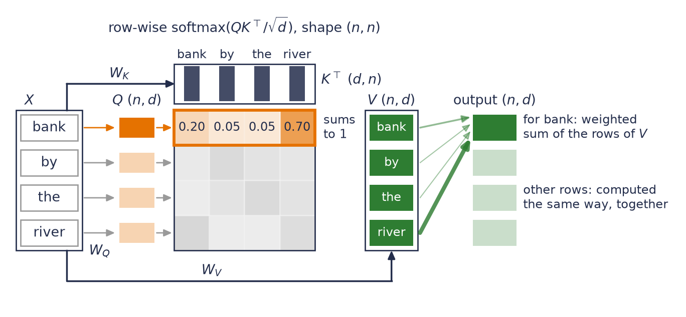
Figure 16.1 follows one query, bank, through the four-token fragment bank by the river: the same sequence supplies the queries, keys, and values, and the query’s row of the \(n\times n\) grid becomes the weights on the rows of \(V\).

Figure 16.1: Self-attention keeps the operator of Chapter 15 and changes only where its inputs come from: one sequence \(X\), through the learned projections \(W_Q\), \(W_K\), \(W_V\), supplies the queries, keys, and values. The query for bank scores every key, itself included, and the row-wise softmax turns the scores into weights that sum to one; the output for bank is the weighted sum of the rows of \(V\) (arrow width shows each weight; the numbers and shading are illustrative). The fainter rows do the same for every other token, together.

Weights were already shared across examples and across space; Chapter 12 made time the third axis of weight sharing. An RNN shares transition parameters across time. Self-attention shares projection parameters across positions and applies the same comparison rule to each permitted query–key pair. The weights in a particular attention row still depend on the content; what is shared is the machinery that produces them.

For one sequence, that comparison rule comes down to one learned matrix. With \(\vect{x}_i^\top\) as row \(i\) of \(X\), substituting the projections gives

\[ \frac{(QK^\top)_{ij}}{\sqrt d} =\frac{\vect{x}_i^\top W_QW_K^\top\vect{x}_j}{\sqrt d}. \]

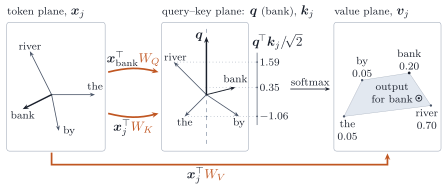
The kernel smoother of Chapter 14 compared a query with a key through a fixed distance and a single bandwidth. Here training sets the \(d\times d\) matrix \(W_QW_K^\top\), which decides which features of the querying token are compared with which features of the token being read. Because \(W_Q\) and \(W_K\) are trained separately, \(W_QW_K^\top\) need not be symmetric, so the score of bank against river need not equal the score of river against bank. Chapter 15 called the learned kernel an analogy for this reason: a classical kernel is symmetric and positive semidefinite, and this score need be neither.¹ Lopsided attention weights are not evidence of that asymmetry. Softmax normalizes each row on its own, so even a symmetric score can give bank’s row most of its weight on river while river’s row spreads its weight across other keys. Figure 16.2 draws one such row, bank’s, to scale in a two-dimensional toy, where each learned matrix appears as what it is, a function from one plane to another, and each score as a signed shadow on the line through the query.

Figure 16.2: Bank’s row of Figure 16.1 as geometry, in a toy with \(d=2\) built to reproduce its illustrative weights. Each plane, drawn to scale, stands in for the \(d\) dimensions of a real model. Orange marks only the learned maps. The query is computed by one, not learned, so it is drawn in black (orange in Figure 16.1), as are bank’s token, key, value and output. Left: each map is a function of a token \(\vect{x}_j^\top\), a row of \(X\). So \(\vect{q}^\top=\vect{x}_{\text{bank}}^\top W_Q\) is bank’s row of \(Q\), and \(\vect{k}_j^\top=\vect{x}_j^\top W_K\) and \(\vect{v}_j^\top=\vect{x}_j^\top W_V\) are the rows of \(K\) and \(V\). Middle: a key’s score \(\vect{q}^\top\vect{k}_j/\sqrt2=\vect{x}_{\text{bank}}^\top W_QW_K^\top\vect{x}_j/\sqrt2\) is its signed shadow on the dashed line through \(\vect{q}\), as in Figure 1.2, times \(\norm{\vect{q}}/\sqrt2\). By and the share one shadow and tie. Right: softmax over this one row gives the weights. The output (ring), the values’ weighted average, lies inside their hull, nearest river. Not shown: the other rows, whether \(W_QW_K^\top\) is symmetric, and what trained maps learn.

All query positions can be evaluated together during training because none waits for a hidden state from the preceding position. That is a structural statement, not a timing result. Dense self-attention still forms \(n^2\) pairwise scores, and autoregressive generation still emits one new token at a time.

Watch the mechanism: reorder the tokens and follow bank's row

Reorder bank, by, the, river as by, river, bank, the. Bank's row of weights follows its query down to slot 2. The keys reorder too: does bank's 0.70 stay in column 3, or follow river's key?

The weights are those of the figure above, for bank, by, the, river: rows are queries, columns are keys, and slots count from 0. Only bank's row is printed; the fainter rows are shading.

\(\operatorname{Attention}(Q,K,V)=\operatorname{softmax}\left(\frac{\class{ba-q}{Q}\class{ba-kt}{K^\top}}{\sqrt d}\right)\class{ba-v}{V}\)

Bank's 0.20 is back on the diagonal, and 0.70 still meets river's value block.

The calculation is readable without playback. Opening this panel loads the optional controls.

One reordering of the chapter's illustrative weights, in bare self-attention with no mask and no position signal; the proof that follows covers every reordering.

Scope and caveats

The reordering (by, river, bank, the) is declared. Every token moves, and the reordering does not reverse itself. The chapter's own audit, later in this section, reorders random vectors in another order; the panel takes none of its numbers and none of its order.

The weights are the figure's illustrative ones. Only bank's row is printed, as in the figure; the other rows are shading.

Rows first, then columns, is a drawing device. The rows-only grid is a real quantity: reordered queries scored against keys still in their old order. But attention on the reordered sequence reorders rows and columns at once, as the one-move glide shows.

Had the value blocks moved while the columns stayed put, bank's 0.70 in column 3 would meet the's value block, and bank's output would change. The panel never draws that state.

One example, not a proof. “Bare” means no mask and nothing tied to slot numbers; the chapter adds both later, and each changes more than addresses.

The palette departs from the figure's house orange, grey and green: here the weights are green, as probabilities, and token names, value blocks and output blocks are blue.

Check yourself. Reorder to the, river, by, bank. In which cells (row, column; slots 0 to 3) do bank's 0.70 and bank's own 0.20 land, and how does bank's row read?

Row 3, bank's new slot: 0.70 follows river's key to (3, 1), and bank's 0.20 lands on the diagonal at (3, 3). The row reads 0.05, 0.70, 0.05, 0.20. Moving the rows alone would leave 0.70 at (3, 3), on bank's own diagonal cell.

Transcript and keyboard help

1. The chapter's order, bank, by, the, river, on both axes: rows are queries, columns are keys, and the slot labels count from 0. Bank's row reads 0.20, 0.05, 0.05, 0.70: bank's 0.20 on its own key and 0.70 on river's. A tick marks each token's weight on itself, and all four ticks sit on the diagonal. A value block sits under each key column, and an output block ends each row.
2. Reorder to by, river, bank, the. The query rows glide first, each with its token name and its output block. Bank's row lands in slot 2, still reading 0.20, 0.05, 0.05, 0.70, and bank's output lands in slot 2 with it. Every tick leaves the diagonal. The columns have not moved.
3. The keys reorder too. Predict: does bank's 0.70 stay in column 3, or follow river's key? Nothing moves while you decide.
4. The key columns glide, each with its token name, and each value block slides beneath its column on the same clock. 0.70 rides river's column to column 1, bank's 0.20 reaches the diagonal at (2, 2), and every tick returns to the diagonal. Bank's output block neither moves nor changes: river's value came along with river's weight.
5. Back to the chapter's order by a brief fade, then the same reordering in one move: rows with their output blocks and columns with their value blocks, on one clock. Each weight travels straight from its old cell to its new one, and every tick slides along the diagonal without leaving it.
6. Queries moved the rows, keys moved the columns, and each value block moved with its key.
7. Bank's row holds the same four weights at new addresses and now reads 0.05, 0.70, 0.20, 0.05 in the new column order. Bank's output sits in slot 2, unchanged.
8. A ghost outline marks where bank's row began, at slot 0, and a thin path runs from 0.70's first cell, (0, 3), to its last, (2, 1). Bank's 0.20 is back on the diagonal, and 0.70 still meets river's value block.

Silent; paused initially; 1.5× playback. Focus the animation pane: Space or K plays/pauses, arrows seek between beats, Home/End jump, Escape pauses. The scrubber and speed menu also work by keyboard. Reduced-motion mode holds each beat's state instead of moving between them.

Permutation symmetry without positional signals or masks

First consider self-attention without positional signals or an attention mask. We will show that permuting the input rows permutes the output rows in the same way. A fixed causal mask changes this setting by assigning different visible prefixes to different positions.

Let \(P\) be an \(n\times n\) permutation matrix, so \(PX\) reorders the tokens. Then

\[ Q'=PQ,\quad K'=PK,\quad V'=PV \]

and therefore

\[ Q'K'^\top=P(QK^\top)P^\top. \]

Write \(S=QK^\top/\sqrt d\); then \(S'=PSP^\top\). Row-wise softmax respects the same simultaneous row-and-column permutation:

\[ \operatorname{softmax}(PSP^\top) =P\operatorname{softmax}(S)P^\top. \]

Putting the pieces together gives

\[ \operatorname{SA}(PX) =P\operatorname{SA}(X). \]

Self-attention is permutation equivariant: permute the inputs and the outputs permute in the same way. It is not permutation invariant; the token outputs do not all become identical. But without another signal, the operator has no basis for distinguishing “first” from “fifth.” A pooled sequence summary can consequently become invariant to order.

In Chapter 9, convolution received locality “for free.” A convolution knows which values are neighbors because its kernel is tied to nearby offsets. Global attention drops that built-in geometry, so position has to be supplied explicitly.

1. Define the reusable helpers: numpy_attention and numpy_positions.
2. Draw five random width-8 tokens, permute them, and find the largest output mismatch, bare and with pe added.
3. Report the permutation-equivariance and fixed-slot differences.

import math
import numpy as np
import matplotlib.pyplot as plt

# [1]
def numpy_attention(x: np.ndarray) -> np.ndarray:
    scores = x @ x.T / math.sqrt(x.shape[-1])
    scores = scores - scores.max(axis=-1, keepdims=True)
    weights = np.exp(scores)
    weights = weights / weights.sum(axis=-1, keepdims=True)
    return weights @ x

def numpy_positions(length: int, width: int) -> np.ndarray:
    position = np.arange(length)[:, None]
    frequency = np.exp(
        np.arange(0, width, 2) * (-math.log(10_000.0) / width)
    )
    pe = np.zeros((length, width))
    pe[:, 0::2] = np.sin(position * frequency)
    pe[:, 1::2] = np.cos(position * frequency)
    return pe

# [2]
rng = np.random.default_rng(6050)
x = rng.normal(size=(5, 8))
permutation = np.array([2, 4, 0, 1, 3])
bare_error = np.abs(
    numpy_attention(x[permutation]) - numpy_attention(x)[permutation]
).max()

pe = numpy_positions(5, 8)
with_position = numpy_attention(x + pe)
fixed_slot_change = np.abs(
    numpy_attention(x[permutation] + pe) - with_position[permutation]
).max()

# [3]
print(f"bare permutation-equivariance error: {bare_error:.2e}")
print(f"fixed-slot difference after adding position: {fixed_slot_change:.3f}")

bare permutation-equivariance error: 2.22e-16
fixed-slot difference after adding position: 1.581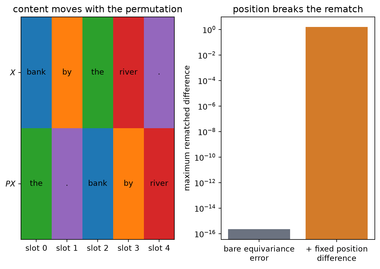

Figure 16.3: The same content is permuted across slots (left). The audit (right) shows bare self-attention rematches after the same output permutation, while fixed positional signals break that rematch.

The first error is numerical roundoff, about \(2.2\times10^{-16}\). Adding a fixed signal to each slot raises the same error to about 1.581 in this example. Position has not been inferred from content; it has been supplied.

16.2 Position as a bank of clocks

The simplest additive code repeats \(i/(n-1)\) in every coordinate. It supplies order, but every position vector lies on the same ray, so the vectors differ in magnitude, not in direction. A binary code supplies more coordinates, yet adjacent integers can flip many bits and have poor locality. These are not impossible designs; they are weak inductive biases for a model that must reason about shifts and distances.

Sinusoidal encoding gives every position a bank of clocks. For even model width \(d\), define

\[ \begin{aligned} \operatorname{PE}(i,2j) &=\sin\left(i\,10000^{-2j/d}\right),\\ \operatorname{PE}(i,2j+1) &=\cos\left(i\,10000^{-2j/d}\right). \end{aligned} \]

Small \(j\) gives a fast clock; large \(j\) gives a slow one. Every sine coordinate is paired with a cosine at the same frequency. The model receives

\[ Z_i=\sqrt d\,E_i+\operatorname{PE}(i), \]

where \(E_i\) is the token embedding. Scaling the embedding keeps its initial magnitude comparable to that of the position vector.

Why pair sine and cosine? For frequency \(\omega\), advancing by offset \(\delta\) is a rotation:

\[ \begin{bmatrix} \sin((i+\delta)\omega)\\ \cos((i+\delta)\omega) \end{bmatrix} = \begin{bmatrix} \cos(\delta\omega)&\sin(\delta\omega)\\ -\sin(\delta\omega)&\cos(\delta\omega) \end{bmatrix} \begin{bmatrix} \sin(i\omega)\\ \cos(i\omega) \end{bmatrix}. \]

The rotation depends on the offset, not the absolute position. This gives learned linear maps a convenient raw material for representing relative shifts. It is a property of the positional pair itself, not a guarantee that arbitrary learned \(W_Q\) and \(W_K\) will preserve or use it.

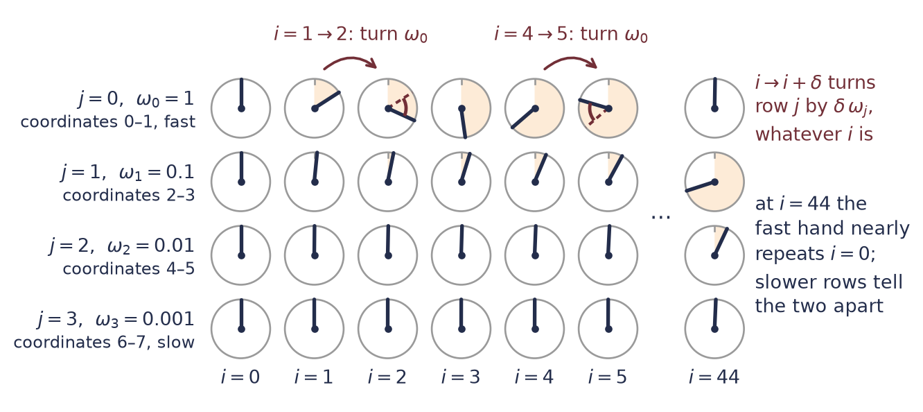
In Figure 16.4, the four clocks of a width-8 code show that one step turns row \(j\) by the same \(\omega_j\) from any start. At \(i=44\) the fast \(j=0\) hand has nearly come back to its angle at \(i=0\), yet the slower clocks still tell positions 44 and 0 apart.

Figure 16.4: Six nearby positions and one far one, read off the four clocks of the width-8 code in the permutation audit. Row \(j\) draws \((\operatorname{PE}(i,2j),\operatorname{PE}(i,2j+1))=(\sin(i\omega_j),\cos(i\omega_j))\) with \(\omega_j=10000^{-2j/d}\), sine horizontal and cosine vertical, so every hand starts straight up and turns clockwise; shading is the angle past the last full turn. In the two dials marked in wine, the dashed hand is the previous position and the arc shows one step turning the fast hand by the same \(\omega_0=1\) radian from two different starts, while at \(i=44\approx7\cdot2\pi\) the fast hand nearly repeats \(i=0\) and only the slower clocks tell the two positions apart.

NoteRotate the queries and keys

Instead of adding the clock coordinates to the token, rotate each query and key directly. If \(R_i\) is the block-diagonal rotation for position \(i\), use \(\widetilde{\vect{q}}_i=R_i\vect{q}_i\) and \(\widetilde{\vect{k}}_j=R_j\vect{k}_j\). Their score becomes

\[ \widetilde{\vect{q}}_i^\top\widetilde{\vect{k}}_j =\vect{q}_i^\top R_i^\top R_j\vect{k}_j =\vect{q}_i^\top R_{j-i}\vect{k}_j. \]

The positional factor now depends on the relative offset \(j-i\). This construction is called rotary positional embedding (RoPE). Content still matters through \(\vect{q}_i\) and \(\vect{k}_j\); RoPE changes how position enters their comparison.

1. Encode 100 positions at width 32, rotate position 13’s pair j = 5 by offset 7, and compute rotation and norm errors.
2. Verify the rotation identity and constant-norm invariant.

# [1]
pe = numpy_positions(100, 32)

delta = 7
j = 5
omega = 10_000 ** (-2 * j / 32)
rotation = np.array([
    [np.cos(delta * omega), np.sin(delta * omega)],
    [-np.sin(delta * omega), np.cos(delta * omega)],
])
pair_i = pe[13, 2 * j : 2 * j + 2]
pair_shifted = pe[13 + delta, 2 * j : 2 * j + 2]
rotation_error = np.abs(rotation @ pair_i - pair_shifted).max()
norm_error = np.abs(np.linalg.norm(pe, axis=1) - 4.0).max()

# [2]
print(f"rotation identity maximum error: {rotation_error:.2e}")
print(f"constant position-vector norm maximum error: {norm_error:.2e}")

rotation identity maximum error: 1.11e-16
constant position-vector norm maximum error: 0.00e+00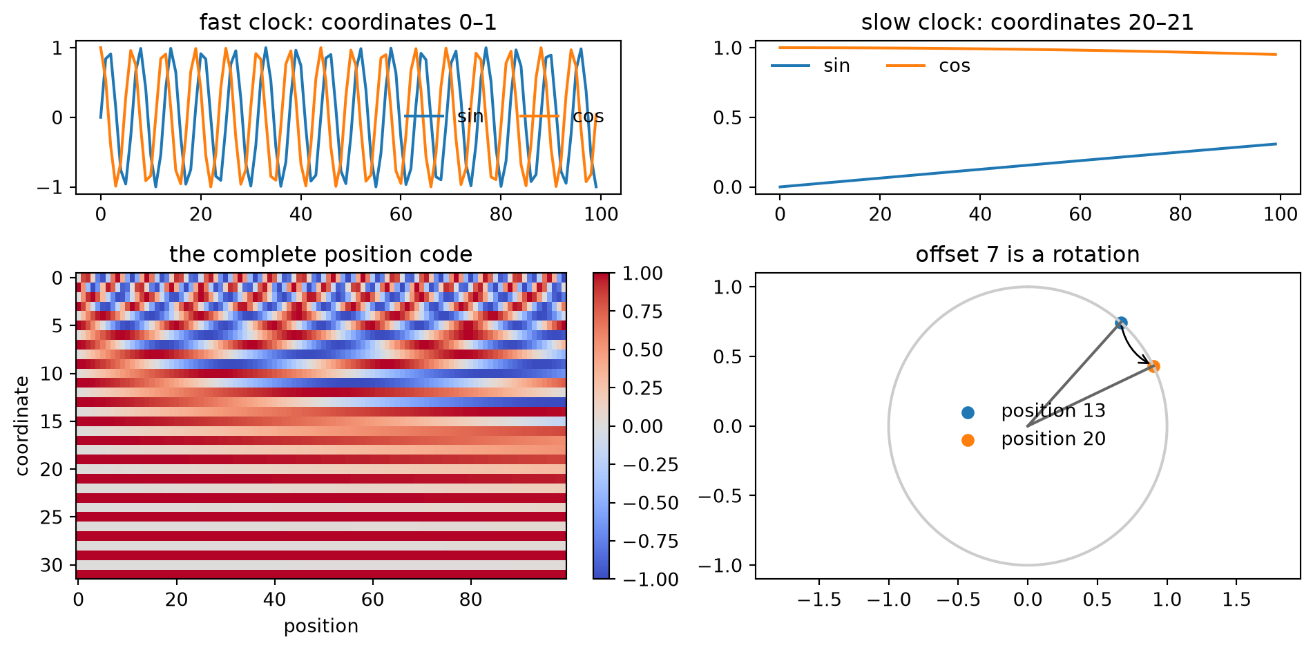

Figure 16.5: Sinusoidal position is a bank of clocks. Fast coordinates track local offsets; slow coordinates vary across longer ranges. Each sine/cosine pair acts like a clock, and a fixed offset rotates that pair by a start-independent angle.

For \(d=32\), each position vector has norm \(\sqrt{d/2}=4\) because every \(\sin^2+\cos^2\) pair contributes one. Adding this vector does not preserve the norm of the combined token representation: the embedding and position vector can reinforce or cancel one another. Layer normalization will soon manage scale at the block level.

16.3 One routing operation, many heads

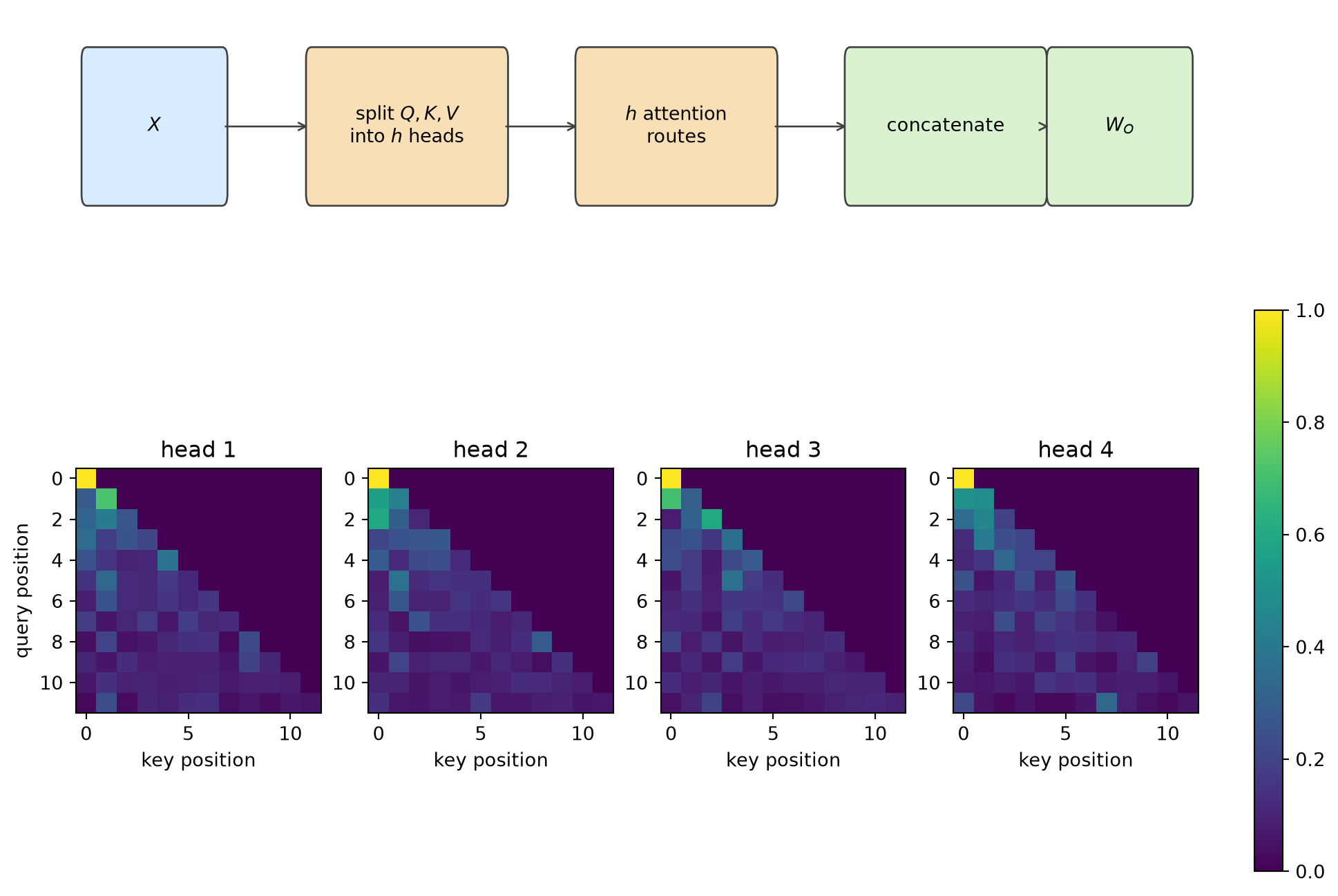
A single attention distribution must make one compromise about what to retrieve. Multi-head attention runs several smaller routing systems in parallel, each with its own projections of the same residual stream. Choose a number of heads \(h\) that divides \(d\), and let \(d_h=d/h\). For each head \(r\),

\[ Q_r=XW_Q^{(r)},\quad K_r=XW_K^{(r)},\quad V_r=XW_V^{(r)}, \]

where \(W_Q^{(r)},W_K^{(r)},W_V^{(r)}\in\mathbb{R}^{d\times d_h}\). The head output is

\[ H_r= \operatorname{softmax}\left( \frac{Q_rK_r^\top}{\sqrt{d_h}}+M \right)V_r. \]

Here \(M\) is the visibility mask defined next; \(M=0\) for unmasked attention.

The complete operation concatenates the heads and mixes them:

\[ \operatorname{MHA}(X) =\operatorname{Concat}(H_1,\ldots,H_h)W_O, \qquad W_O\in\mathbb{R}^{d\times d}. \]

Tensor shapes are the safest implementation guide:

\[ (B,n,d) \to(B,h,n,d_h) \to(B,h,n,n) \to(B,h,n,d_h) \to(B,n,d). \]

Scaling uses \(\sqrt{d_h}\), not \(\sqrt d\), because a head’s dot product sums \(d_h\) terms, and the previous chapter’s variance argument applies to that sum. With fixed \(d\), splitting into heads does not multiply the leading projection count: \(W_Q,W_K,W_V,W_O\) together contribute about \(4d^2\) weights regardless of \(h\). Heads divide the model width among themselves; they do not each receive a fresh width-\(d\) model.

The mask is part of the model

Chapter 13 called masking the rule that tells a model which positions it may not look at. Here that rule is causal: position \(i\) may use tokens at positions \(j\le i\) but must not inspect future tokens \(j>i\). Rows are queries and columns are keys, so the forbidden region is the strict upper triangle. We add

\[ M_{ij}= \begin{cases} 0,&j\le i,\\ -\infty,&j>i \end{cases} \]

before softmax. Replacing forbidden probabilities with zero afterward would leave the remaining row unnormalized. Adding \(-\infty\) first gives the same row as zeroing those probabilities and then dividing the rest by their sum. Each row becomes the unmasked row conditioned on the event \(j\le i\). Masking every key in a row is invalid; softmax would receive only negative infinity. Here the diagonal remains visible: the representation at a character may use that character while predicting the next one.

1. Define the CausalMultiHeadAttention module.
2. Fix the seed, run 12 random width-32 tokens through a 4-head module, and build the strict upper-triangle future mask.
3. Implement causal multi-head attention and audit its mask.

import torch
from torch import nn
torch.set_num_threads(4)  # pinned: results depend on the CPU thread count

# [1]
class CausalMultiHeadAttention(nn.Module):
    def __init__(self, width: int, heads: int) -> None:
        super().__init__()
        if width % heads != 0:
            raise ValueError("width must be divisible by heads")
        self.heads = heads
        self.head_width = width // heads
        self.qkv = nn.Linear(width, 3 * width)
        self.project = nn.Linear(width, width)
        nn.init.xavier_uniform_(self.qkv.weight)
        nn.init.zeros_(self.qkv.bias)

    def forward(self, x: torch.Tensor, return_weights: bool = False):
        batch, length, width = x.shape
        qkv = self.qkv(x)
        qkv = qkv.reshape(
            batch, length, 3, self.heads, self.head_width
        ).permute(2, 0, 3, 1, 4)
        q, k, v = qkv.unbind(dim=0)
        scores = q @ k.transpose(-2, -1) / math.sqrt(self.head_width)
        forbidden = torch.triu(
            torch.ones(length, length, dtype=torch.bool, device=x.device),
            diagonal=1,
        )
        scores = scores.masked_fill(forbidden, float("-inf"))
        weights = torch.softmax(scores, dim=-1)
        routed = weights @ v
        routed = routed.transpose(1, 2).reshape(batch, length, width)
        output = self.project(routed)
        if return_weights:
            return output, weights
        return output

# [2]
torch.manual_seed(6050)
demo_attention = CausalMultiHeadAttention(width=32, heads=4)
demo_x = torch.randn(1, 12, 32)
_, demo_weights = demo_attention(demo_x, return_weights=True)

future = torch.triu(torch.ones(12, 12, dtype=torch.bool), diagonal=1)
# [3]
assert demo_weights[0, :, future].max().item() == 0.0
assert torch.allclose(
    demo_weights.sum(dim=-1),
    torch.ones_like(demo_weights.sum(dim=-1)),
    atol=1e-6,
)

Figure 16.6: Multi-head attention splits, routes in parallel, concatenates, and projects (top). In the untrained causal heads below, every query row sums to one and every future key has exactly zero weight.

1. Report the causal-mask and normalization audit.

# [1]
print("maximum forbidden attention:", demo_weights[0, :, future].max().item())
print(
    "maximum row-sum error:",
    (demo_weights.sum(dim=-1) - 1).abs().max().item(),
)

maximum forbidden attention: 0.0
maximum row-sum error: 1.1920928955078125e-07

The assertions are part of the derivation. A visually plausible triangle can still be transposed, shifted by one, or applied after softmax. Executable shape and normalization checks catch those errors, before training can disguise them.

The mask changes visibility, not dense computation. The implementation still forms all \(n^2\) scores and stores \(Bhn^2\) attention weights, alongside roughly \(Bnd^2\) projection work and \(Bndd_{ff}\) work in the FFN. Self-attention shortens the graph path between distant tokens to one routing step, but “one step away” is not “constant runtime.” Appendix C returns to this \(n^2\) cost through Roofline analysis and FlashAttention’s I/O-aware schedule.

16.4 Build a Transformer block

Attention routes information between token positions. A Transformer block needs two more ingredients: a stable path through depth and a nonlinear computation at each position.

The residual stream

Chapter 10 introduced the residual stream: every block reads the stream and writes a correction back. If a sublayer computes \(F(x)\), the residual update is

\[ x\leftarrow x+F(x). \]

The identity branch provides a direct route for representations and gradients while the learned branch proposes a correction. It makes deep optimization more tractable; it does not guarantee that gradients can never vanish or explode.

Layer normalization controls each token’s feature scale. For one token vector \(x\in\mathbb{R}^{d}\),

\[ \mu=\frac1d\sum_{k=1}^{d}x_k,\qquad \sigma^2=\frac1d\sum_{k=1}^{d}(x_k-\mu)^2, \]

\[ \operatorname{LN}(x)_k =\gamma_k\frac{x_k-\mu}{\sqrt{\sigma^2+\epsilon}}+\beta_k, \qquad \gamma,\beta\in\mathbb{R}^d. \]

This is Chapter 10’s normalization equation applied along a different axis. Chapter 10’s BatchNorm2d used batch and spatial axes for each channel. LayerNorm flips to the feature axis of each token: it computes statistics across the features within one token, without aggregating statistics across other tokens or examples. Its calculation is the same at training and evaluation time. Before the learned \(\gamma\) and \(\beta\), the vector is approximately zero mean and unit variance. After applying them, that claim need not remain true. Geometrically, before \(\gamma\) and \(\beta\), subtracting \(\mu\) from every entry removes \(\mu(1,\ldots,1)\), the projection of \(x\) onto the all-ones vector. Dividing by \(\sqrt{\sigma^2+\epsilon}\) then brings the squared length to \(d\sigma^2/(\sigma^2+\epsilon)\). When \(\sigma^2\) is much larger than \(\epsilon\), this is just under \(d\), so the normalized token lies just inside the sphere of radius \(\sqrt d\).

1. Apply layer_norm to four width-4 tokens with different offsets and scales, then take each token’s mean and variance.
2. Verify LayerNorm centers and scales each token independently.

# [1]
audit = torch.tensor([
    [[1.0, 3.0, 5.0, 7.0], [40.0, 50.0, 60.0, 70.0]],
    [[-3.0, 1.0, 5.0, 9.0], [2.0, 2.5, 3.0, 3.5]],
])
normalized = nn.functional.layer_norm(audit, (4,))
token_means = normalized.mean(dim=-1)
token_vars = normalized.var(dim=-1, unbiased=False)
# [2]
assert token_means.abs().max().item() < 1e-6
assert (token_vars - 1).abs().max().item() < 1e-4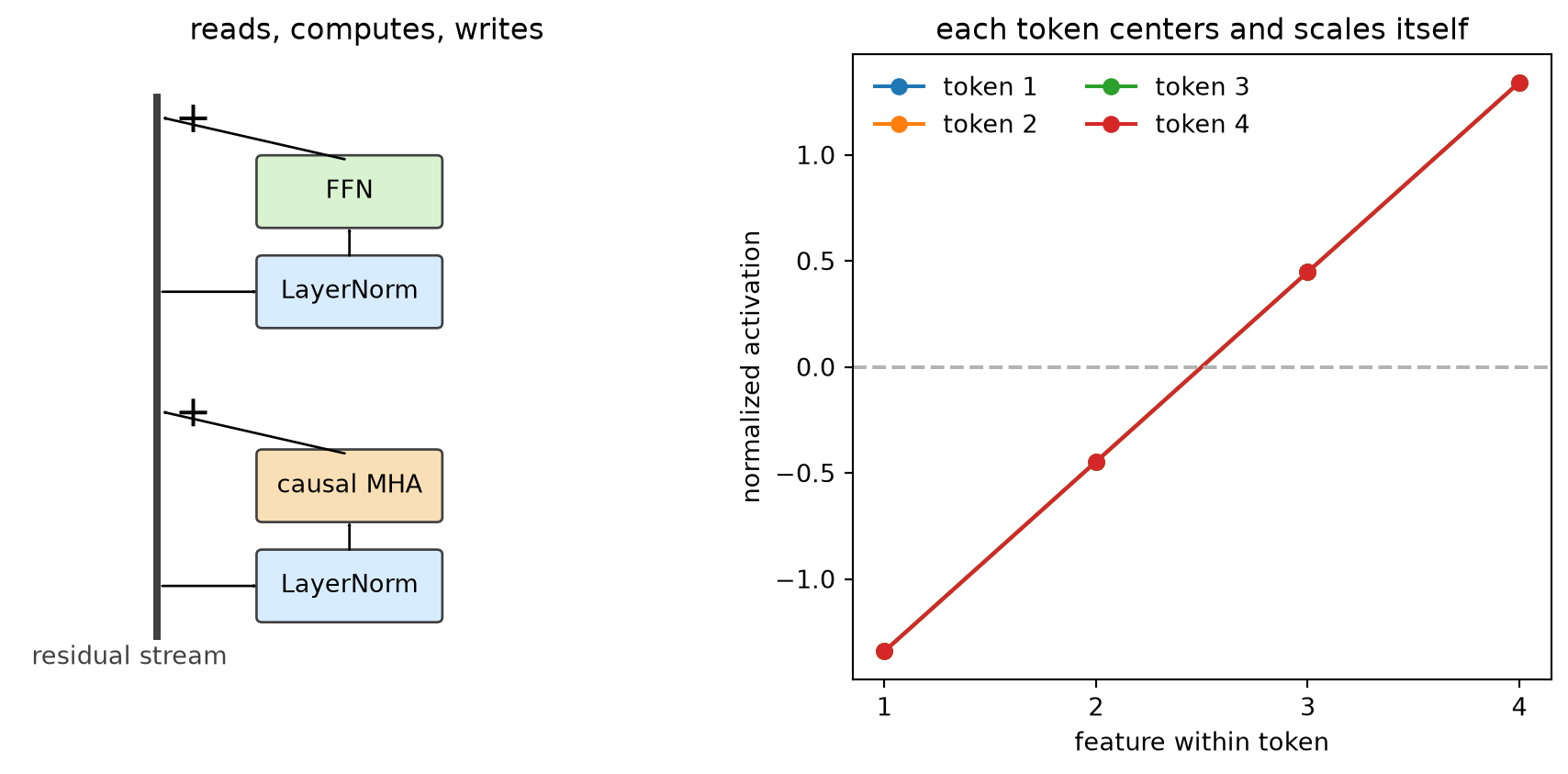

Figure 16.7: A pre-LayerNorm Transformer block as two read–compute–write stages. The residual stream carries each token directly across both additions while LayerNorm feeds a normalized view to causal multi-head attention and then the position-wise FFN. The audit at right shows what LayerNorm changes: four tokens with different offsets and scales become the same centered, unit-variance profile before the learned affine rescaling.

Watch the mechanism: BatchNorm down, LayerNorm across

BatchNorm and LayerNorm apply the same formula. If a neighboring token's values change, does this token's normalized output change too?

First compare the groups that share statistics. Then follow the audit's first token as its feature profile shifts and rescales. Last comes a test: a neighboring token doubles. Decide beforehand what will move.

\( \mu=\dfrac1d\class{la-pool-term}{\sum_k}\featurepart{x_k} \) \( \predictionpart{z_k}=\dfrac{\class{la-center-term}{\featurepart{x_k}-\mu}}{\class{la-scale-term}{\sqrt{\sigma^2+\epsilon}}} \) \( \operatorname{Var}(\predictionpart{z})=\dfrac{\sigma^2}{\sigma^2+\epsilon},\quad\epsilon=10^{-5}>0 \)

A token's LayerNorm result does not depend on batchmates or sequence length; BatchNorm's statistics do. Before learned scale and shift.

The calculation is readable without playback. Opening this panel loads the optional controls.

The token tensor is not an image: its vertical bracket shows temporal BatchNorm during training, pooling examples and positions separately for each feature.

Scope and caveats

The separate CNN sketch holds one channel fixed and pools images and spatial positions. The LayerNorm profile keeps a fixed value ruler; its dashed blue ghost is the raw first token. Each row normalizes separately, before learned scale and shift. Positive epsilon makes the near-unit variance approximate. The closing test is a computed variant of the audit tensor, not new data: the neighboring token (40, 50, 60, 70) is doubled and the same LayerNorm is run again. Of BatchNorm, only the pooled feature-1 mean is shown, 10 before and 20 after; no BatchNorm output is computed. While the neighbor's numerals move they are rounded to whole numbers. The test holds this token's own features fixed; attention may already have mixed context into them.

Why BatchNorm fits images and LayerNorm fits sequences

Why sharing can fit a CNN. One convolutional channel measures the same kind of feature across a regular spatial grid. BatchNorm shares that channel's training statistics across images and positions, the \(N,H,W\) axes. Matching image sizes make dense minibatches convenient; fixed image size is not a requirement of BatchNorm itself. By default, evaluation uses running statistics collected during training.

Why token-local statistics fit variable lengths. Ordinary temporal BatchNorm pools the \(B,T\) axes. Unmasked padding enters those statistics; even masked pooling gives longer sequences more entries. LayerNorm instead pools a token's features: sequence length can vary while feature width stays fixed. With that token's input features held fixed, padding elsewhere or different batchmates cannot change its LayerNorm result. It uses the same calculation in training and evaluation. Attention and loss masks are still needed.

Check yourself. Multiply the first token's four features by 10, to (10, 30, 50, 70). What is its LayerNorm output?

The same: (−1.342, −0.447, 0.447, 1.342), up to the tiny effect of ε. The mean and the standard deviation both grow tenfold and cancel. LayerNorm removes each token's own offset and scale, whatever the other tokens are doing.

Transcript and keyboard help

1. The audit has two examples, two tokens per example, and four features per token. The opening vertical bracket selects one feature across every example and token, the group used by temporal BatchNorm during training. A separate nonnumeric CNN sketch connects two images' feature maps for one channel to shared statistics across images and spatial positions. It does not reinterpret the token tensor as images.
2. At five seconds the axis begins to change. One highlight turns, over two and a half seconds ending at ten seconds, from that vertical feature column into the horizontal row of example 1, token 1: 1, 3, 5, 7. It pivots about the one cell the two groups share, this token's own feature 1, so the reader follows a single rectangle rather than a swap. The column it leaves stays on the picture as a muted dashed outline until the closing test, and its numerals return to gray; the persistent axis key keeps both directions explicit. The token's raw profile appears as the turn begins, taking the place of the CNN sketch.
3. This row's mean is 4 and its population variance is 5. None of the other tokens enters either calculation.
4. Subtract 4 from every feature. The same profile translates to minus 3, minus 1, 1, 3 and has mean zero.
5. Divide every centered feature by the square root of 5 plus the positive stability constant, approximately 2.236.
6. The resulting values are approximately minus 1.342, minus 0.447, 0.447, 1.342. Their variance is approximately 0.999998, not exactly one.
7. At thirty seconds both groups are outlined on the same tensor: BatchNorm's feature 1 column and LayerNorm's first-token row. Under the plot, one number line carries two pointers: this token's mean, 4, above it, and feature 1's pooled mean, 10, below it. The caption asks for a prediction: the neighboring token, example 1 token 2, is about to double. Then its values rise from 40, 50, 60, 70 to 80, 100, 120, 140. The pooled-mean pointer slides from 10 to 20, because the changed value, 40 to 80, lies inside BatchNorm's column. The token's own mean pointer and its normalized profile do not move: no changed value lies inside LayerNorm's row. LayerNorm was run again on the changed tensor to draw that unmoved profile.
8. A token's LayerNorm result does not depend on its batchmates or on sequence length; BatchNorm's training statistics do. The final frame keeps both outlines, the doubled row, the pooled mean's move from 10 to 20, and the unmoved profile −1.342, −0.447, 0.447, 1.342. This is before learned scale and shift. A positive stability constant slightly changes the variance. Default BatchNorm evaluation uses running statistics; LayerNorm uses the same token-local calculation in training and evaluation. With that token's features held fixed, padding elsewhere does not enter its normalization. Attention may already have mixed context into those features; attention and loss masks remain necessary. Naive temporal BatchNorm pooling in a causal model can also include future positions.

Silent; paused initially; 1.5× playback. Focus the animation pane: Space or K plays/pauses, arrows seek between beats, Home/End jump, Escape pauses. The scrubber and speed menu also work by keyboard. Reduced-motion mode holds each beat's state instead of moving between them.

1. Report the per-token LayerNorm audit.

# [1]
print("maximum absolute token mean:", token_means.abs().max().item())
print("maximum token variance error:", (token_vars - 1).abs().max().item())

maximum absolute token mean: 0.0
maximum token variance error: 3.2067298889160156e-05

The original Transformer normalized after each residual addition:

\[ x\leftarrow\operatorname{LN}(x+\operatorname{MHA}(x)),\qquad x\leftarrow\operatorname{LN}(x+\operatorname{FFN}(x)). \]

Our small experiment uses the now-common pre-LayerNorm arrangement:

\[ \begin{aligned} x&\leftarrow x+\operatorname{MHA}(\operatorname{LN}(x)),\\ x&\leftarrow x+\operatorname{FFN}(\operatorname{LN}(x)). \end{aligned} \]

Post-LayerNorm normalizes after each residual addition, where the original ResNet block of Chapter 10 applied its final ReLU. Pre-LayerNorm moves the normalization into the learned branch, as pre-activation ResNets did with that ReLU. Xiong et al. argued that the post-LayerNorm placement is one reason the original Transformer needed warmup (Chapter 4), which raises the learning rate gradually from a small value. In their analysis at initialization, post-LayerNorm gives large gradients to the parameters of the layers nearest the output. Starting at the full learning rate can then make training unstable, and warmup keeps the first steps small. In their experiments, pre-LayerNorm Transformers trained without warmup did about as well as post-LayerNorm baselines trained with it.

Pre-LayerNorm leaves an unobstructed identity route along the residual stream and often improves optimization at initialization. This is an implementation choice, not a universal theorem that post-LayerNorm fails or that pre-LayerNorm eliminates every need for careful optimization.

RMSNorm keeps the scale control but omits mean subtraction:

\[ \operatorname{RMSNorm}(\vect{x}) =\vect{g}\odot \frac{\vect{x}} {\sqrt{\frac{1}{d}\sum_{j=1}^{d}x_j^2+\epsilon}}. \]

It normalizes each token by its root-mean-square magnitude and retains a learned per-feature scale \(\vect{g}\). Before \(\vect{g}\), it rescales \(\vect{x}\) to length about \(\sqrt d\), as LayerNorm does, but leaves the projection onto the all-ones vector in place. This removes one statistic from the computation; it does not imply universal superiority over LayerNorm. Architecture, optimizer, dtype, and scale still determine the observed trade-off.

The position-wise feedforward network

After tokens communicate through attention, the same two-layer network processes each position independently:

\[ \operatorname{FFN}(z) =W_2\operatorname{ReLU}(W_1z+b_1)+b_2. \]

Here \(W_1\in\mathbb{R}^{d_{ff}\times d}\), \(b_1\in\mathbb{R}^{d_{ff}}\), \(W_2\in\mathbb{R}^{d\times d_{ff}}\), and \(b_2\in\mathbb{R}^{d}\).

If \(w_{1j}^\top\) is row \(j\) of \(W_1\) and \(v_j\) is column \(j\) of \(W_2\), the same operation can be written

\[ \operatorname{FFN}(z) =\sum_j [w_{1j}^\top z+b_{1j}]_+\,v_j+b_2. \]

This form suggests reading the FFN as an associative memory. Each first-layer row tests whether the current representation lies in a learned half-space; its positive activation controls how much of the corresponding output vector is written. Empirically, Transformer FFNs can behave like key-value memories. The analogy has limits; the selectors are half-spaces rather than point anchors, the coefficients do not sum to one, and the operation is not literally kernel regression or a normalized lookup.

The complete block therefore alternates two kinds of computation:

1. causal multi-head attention moves information between positions; and
2. the FFN transforms information within each position.

Residual additions keep both results in one shared stream: a common workspace that survives the full stack.

NoteWhat attention alone does to a stack of tokens

An attention layer replaces each token’s vector with a weighted average of the value vectors, with nonnegative weights that add up to one. An average lies between the vectors it averages, so unless rows put nearly all of their weight on single tokens, the outputs sit closer together than the values did. Without the residual additions and the FFN, a second layer averages those averages. In a stack of such layers, every position ends up carrying nearly the same vector, and whatever distinguished one token from another is averaged away.

Dong, Cordonnier, and Loukas bound how fast this happens in unmasked attention. When the query, key, and value matrices are small enough in norm and the tokens already lie close together, their bound on the distance to a state with all token rows equal shrinks doubly exponentially with depth, the exponent tripling at each layer. Their experiments find the same rapid collapse in three pretrained Transformer language models once the residuals are removed.

The residual update \(x\leftarrow x+F(x)\) keeps a path around every attention layer. The differences the tokens arrive with pass through each sum unchanged, and attention only adds its average to them, so the collapse is no longer forced. The FFN cannot do this on its own. It acts on each position separately, so two identical tokens leave it identical. In their analysis, an FFN that can stretch the remaining differences slows the collapse but does not remove it. In Chapter 10, residuals made a deep stack easier to optimize. In a Transformer they do an additional job before any gradient is computed: they keep the tokens distinct.

16.5 From the original Transformer to this experiment

The 2017 Transformer was an encoder–decoder system for translation. Its encoder stack uses unmasked self-attention to build a representation of the source sentence. Its decoder stack uses causal self-attention over the partial target, then cross-attention whose queries come from the decoder while keys and values come from the encoder. In compact form:

\[ \begin{array}{lll} \text{encoder:}&X_s\to\text{self-attention}\to\text{FFN},\\ \text{decoder:}&X_t\to\text{causal self-attention} \to\text{cross-attention to encoder}\to\text{FFN}. \end{array} \]

The book-corpus task predicts the next character from earlier characters. It has no separate source sentence, so the encoder and cross-attention are unnecessary. What remains, a decoder-only causal Transformer, has token plus position embeddings, two pre-LayerNorm blocks, a final LayerNorm, and a linear map to vocabulary logits. The logits go directly to cross-entropy. Softmax belongs inside attention and, later, inside sampling, not between the output layer and the loss.

16.6 The book reads itself, again

We keep every setting that both architectures can share. Chapter 12 trained on a committed snapshot of Chapters 1–6 and 8–10 with executable code cells and HTML comments removed: 148,594 characters, vocabulary 104, a contiguous 90/10 split, 100-character windows, batch size 64, and 2,501 updates with Adam at learning rate 0.002 and gradient clipping at norm 1. The snapshot keeps later copyedits from moving the benchmark. The held-out metric resets state at each fixed window.

The two architectures cannot be made identical (one has recurrent gates and the other has attention blocks), but the training targets each one sees can be. The code below reconstructs Chapter 12’s exact random-window schedule, then gives both Transformer variants the same initial weights and all 16,006,400 target characters in the same order. We have inspected the held-out tail repeatedly across chapters, so we treat it as a stable validation benchmark, not a newly sealed test set.

1. Implement the tiny Transformer: positions, block, model.

# [1]
def sinusoidal_positions(length: int, width: int) -> torch.Tensor:
    position = torch.arange(length, dtype=torch.float32).unsqueeze(1)
    frequency = torch.exp(
        torch.arange(0, width, 2, dtype=torch.float32)
        * (-math.log(10_000.0) / width)
    )
    table = torch.zeros(length, width)
    table[:, 0::2] = torch.sin(position * frequency)
    table[:, 1::2] = torch.cos(position * frequency)
    return table

class TransformerBlock(nn.Module):
    def __init__(self) -> None:
        super().__init__()
        self.norm1 = nn.LayerNorm(WIDTH)
        self.attention = CausalMultiHeadAttention(WIDTH, HEADS)
        self.norm2 = nn.LayerNorm(WIDTH)
        self.ff = nn.Sequential(
            nn.Linear(WIDTH, FF_WIDTH),
            nn.ReLU(),
            nn.Linear(FF_WIDTH, WIDTH),
        )

    def forward(self, x: torch.Tensor, return_weights: bool = False):
        if return_weights:
            attended, weights = self.attention(self.norm1(x), True)
            x = x + attended
            return x + self.ff(self.norm2(x)), weights
        x = x + self.attention(self.norm1(x))
        return x + self.ff(self.norm2(x))

class TinyTransformerLM(nn.Module):
    def __init__(self, vocab: int, positions: bool) -> None:
        super().__init__()
        self.positions = positions
        self.token_embedding = nn.Embedding(vocab, WIDTH)
        nn.init.normal_(
            self.token_embedding.weight,
            mean=0.0,
            std=1 / math.sqrt(WIDTH),
        )
        self.blocks = nn.ModuleList(
            [TransformerBlock() for _ in range(BLOCKS)]
        )
        self.final_norm = nn.LayerNorm(WIDTH)
        self.output = nn.Linear(WIDTH, vocab)
        self.register_buffer(
            "position_table",
            sinusoidal_positions(CONTEXT, WIDTH),
            persistent=False,
        )

    def forward(self, tokens: torch.Tensor, return_weights: bool = False):
        length = tokens.shape[1]
        x = self.token_embedding(tokens) * math.sqrt(WIDTH)
        if self.positions:
            x = x + self.position_table[:length]
        maps = []
        for block in self.blocks:
            if return_weights:
                x, weights = block(x, True)
                maps.append(weights)
            else:
                x = block(x)
        logits = self.output(self.final_norm(x))
        return (logits, maps) if return_weights else logits

The paired protocol is the experimental design. Both variants share windows and initial tensors:

1. Redraw Chapter 12’s window schedule, clone one Transformer initialization, and hash both.
2. Implement the paired protocol: shared schedule, identical initial tensors.

# Reconstruct the random-number state immediately after Chapter 12 created
# its LSTM, then draw that chapter's complete minibatch-start schedule.
# [1]
torch.manual_seed(SEED)
_ = HistoricalCharLSTM(len(chars))
schedule_generator = torch.Generator()
schedule_generator.set_state(torch.random.get_rng_state())
starts = torch.randint(
    0,
    len(train_data) - CONTEXT - 1,
    (UPDATES, BATCH),
    generator=schedule_generator,
)

# The two Transformer variants begin with exactly the same tensors.
torch.manual_seed(SEED)
base_model = TinyTransformerLM(len(chars), positions=True)
initial_state = {
    name: value.clone() for name, value in base_model.state_dict().items()
}
initial_hash = state_digest(initial_state)
schedule_hash = hashlib.sha256(starts.numpy().tobytes()).hexdigest()

# [2]
print(f"corpus: 9 chapters, {len(text):,} characters, vocab {len(chars)}")
print(
    f"deterministic split: {len(train_data):,} train / "
    f"{len(valid_data):,} held out"
)
print(
    f"Transformer parameters: "
    f"{sum(parameter.numel() for parameter in base_model.parameters()):,}"
)
print(f"first eight window starts: {starts[0, :8].tolist()}")
print(f"initial tensors: {initial_hash[:12]}…")
print(f"window schedule: {schedule_hash[:12]}…")

corpus: 9 chapters, 148,594 characters, vocab 104
deterministic split: 133,734 train / 14,860 held out
Transformer parameters: 132,488
first eight window starts: [24368, 94128, 60074, 121547, 118001, 4396, 17011, 8495]
initial tensors: 4d2f7f434cb5…
window schedule: e470a091bd50…

The model has 132,488 trainable parameters, 736 fewer than Chapter 12’s 133,224. That difference is only 0.55%, close enough to remove model size as an easy explanation. The model width is 84, split into four 21-dimensional heads; each of the two FFNs expands to 168 features. We initialize token embeddings with coordinate standard deviation \(1/\sqrt d\) before the displayed \(\sqrt d\) scaling, so their coordinates and the sinusoidal coordinates begin on comparable scales. ModuleList registers the two repeated blocks with the model. The nonpersistent position buffer moves with the model but is neither optimized nor included in the state-dictionary fingerprint; its contents follow deterministically from the displayed formula. There is no dropout, so resetting the trainable/state-dictionary tensors and window schedule makes the positional ablation exact and repeatable.

TipOne seed call was not enough

Calling the same random seed before both training runs would not, by itself, prove that they saw the same windows. Model construction consumes random numbers, and different construction paths can silently shift every later draw. We precompute the full start-index tensor with an explicit generator and copy one saved initialization into both models. We also print fingerprints for both artifacts.

We import Chapter 12’s training and evaluation code unchanged. The trainer’s signature:

1. Reuse the shared trainer through its explicit model, data, schedule, and optimization interface.

# [1]
def fit_next_token(
    model: nn.Module,
    data: torch.Tensor,
    *,
    vocab: int,
    context: int = 100,
    batch: int = 64,
    steps: int = 2501,
    lr: float = 2e-3,
    clip: float = 1.0,
    schedule: list[torch.Tensor] | None = None,
    log_every: int = 500,
    log_decimals: int = 2,
) -> tuple[nn.Module, list[tuple[int, float]]]:

… the body matches Listing 12.1; only the new pieces are printed below.

1. Chapter 12’s trainer, imported: only the deltas printed.

from dlbook.training import fit_next_token      # Listing 12.1, Ch. 12
from dlbook.evaluation import fixed_window_loss  # Listing 12.2, Ch. 12

# [1]
def train_transformer(
    positions: bool,
) -> tuple[nn.Module, list[tuple[int, float]]]:
    net = TinyTransformerLM(len(chars), positions=positions)
    net.load_state_dict(initial_state, strict=True)  # paired start: same tensors
    assert state_digest(net.state_dict()) == initial_hash
    return fit_next_token(
        net, train_data, vocab=len(chars),
        schedule=starts,                 # minibatch order is protocol, not chance
        log_every=250, log_decimals=4,
    )

@torch.no_grad()
def transformer_sample(
    net: nn.Module,
    prompt: str,
    n: int = 300,
    temperature: float = 0.8,
) -> str:
    net.eval()
    generator = torch.Generator().manual_seed(1_406_050)
    tokens = [stoi.get(char, 0) for char in prompt]
    for _ in range(n):
        context = torch.tensor(tokens[-CONTEXT:]).unsqueeze(0)
        probabilities = F.softmax(
            net(context)[0, -1] / temperature, dim=-1
        )
        next_token = torch.multinomial(
            probabilities, 1, generator=generator
        ).item()
        tokens.append(next_token)
    return "".join(chars[index] for index in tokens)

1. Train the positional Transformer.
2. Print the positional model’s fixed-window train and held-out losses.

# [1]
position_model, position_curve = train_transformer(positions=True)
position_train_loss = fixed_window_loss(position_model, train_data, vocab=len(chars))
position_valid_loss = fixed_window_loss(position_model, valid_data, vocab=len(chars))
# [2]
print(f"fixed-window train loss: {position_train_loss:.4f}")
print(f"fixed-window held-out loss: {position_valid_loss:.4f}")

step    0   loss 4.7550
step  250   loss 2.1850
step  500   loss 1.7159
step  750   loss 1.5176
step 1000   loss 1.3955
step 1250   loss 1.3444
step 1500   loss 1.2813
step 1750   loss 1.2386
step 2000   loss 1.1708
step 2250   loss 1.1525
step 2500   loss 1.1083
fixed-window train loss: 1.1132
fixed-window held-out loss: 1.9190

1. Repeat with position removed and everything else fixed.
2. Print the no-position model’s fixed-window train and held-out losses.

# [1]
no_position_model, no_position_curve = train_transformer(positions=False)
no_position_train_loss = fixed_window_loss(
    no_position_model, train_data, vocab=len(chars)
)
no_position_valid_loss = fixed_window_loss(
    no_position_model, valid_data, vocab=len(chars)
)
# [2]
print(f"fixed-window train loss: {no_position_train_loss:.4f}")
print(f"fixed-window held-out loss: {no_position_valid_loss:.4f}")

step    0   loss 4.7289
step  250   loss 2.4955
step  500   loss 2.3612
step  750   loss 2.2436
step 1000   loss 2.2153
step 1250   loss 2.1826
step 1500   loss 2.0792
step 1750   loss 1.9876
step 2000   loss 1.9527
step 2250   loss 1.8986
step 2500   loss 1.8435
fixed-window train loss: 1.8672
fixed-window held-out loss: 2.3405

1. Store Chapter 12’s LSTM held-out loss, 1.888110429, as lstm_valid_loss.
2. Report the positional improvement and LSTM gap.

# [1]
lstm_valid_loss = 1.888110429

# [2]
improvement = no_position_valid_loss - position_valid_loss
relative = improvement / no_position_valid_loss
lstm_gap = position_valid_loss - lstm_valid_loss
print(
    f"position improvement: {improvement:.4f} loss "
    f"({relative:.1%} relative)"
)
print(f"positional Transformer minus LSTM: {lstm_gap:.4f} loss")

position improvement: 0.4214 loss (18.0% relative)
positional Transformer minus LSTM: 0.0309 loss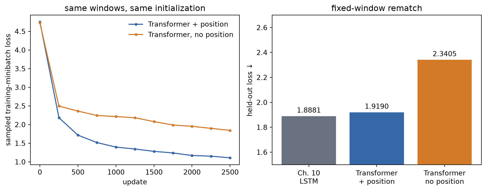

Figure 16.8: Matched training curves (left) and fixed-window held-out loss (right). Position helps in this seed, while the Chapter 12 LSTM has the lowest held-out loss of the three models.

The positional model finishes at 1.1132 on a deterministic pass over the training text and 1.9190 on the held-out tail. Removing position raises those values to 1.8672 and 2.3405. Position lowers held-out loss by 0.4214, or 18.0% relative to the no-position variant.

WarningWhat this matched run can and cannot show

The causal mask already gives a position some weak structural information: row \(i\) sees a prefix of length \(i+1\), and stacked layers can propagate clues from those nested prefixes. That is why the no-position model does better than a purely orderless caricature might suggest. Haviv et al. trained much larger causal language models without positional encodings. Their held-out loss came close to that of models with sinusoidal encoding, and the gap shrank as the models grew. In their no-position models, a small network trained on the internal representations could still predict each token’s approximate position, and the authors proposed that the causal mask supplies this information. Fixed sinusoidal encoding still produces a large improvement in this run.

But Chapter 12’s LSTM remains ahead by 0.0309 held-out loss, or 1.64%. At 100 characters of context and roughly 133,000 parameters, the LSTM has lower held-out loss in this run. This comparison matches corpus, parameter scale, updates, minibatch order, optimizer, clipping, and evaluation. It does not match internal architecture, and it does not show that either model reached its own tuned optimum. We did not repeat the comparison across initialization seeds, so the 0.4214 and 0.0309 gaps are a controlled case study, not an estimate of an average effect.

What did the heads route?

An attention map records routing weights, not reasons, confidence, or a guaranteed explanation of a prediction. Still, inspecting real learned maps can verify the mask and reveal the kinds of patterns a trained model happened to use. The next cell sends the prompt The gradient through the positional model and plots the second block’s four heads.

1. Run the prompt through the positional model and assert the last block’s causal mask and unit row sums.
2. Audit causal masking and row normalization.

# [1]
prompt = "The gradient "
prompt_tokens = torch.tensor([[stoi[char] for char in prompt]])
position_model.eval()
with torch.no_grad():
    _, learned_maps = position_model(prompt_tokens, return_weights=True)
learned = learned_maps[-1][0]

future = torch.triu(
    torch.ones(len(prompt), len(prompt), dtype=torch.bool), diagonal=1
)
assert learned[:, future].max().item() == 0.0
assert torch.allclose(
    learned.sum(dim=-1),
    torch.ones_like(learned.sum(dim=-1)),
    atol=1e-6,
)

# [2]
print("maximum future attention:", learned[:, future].max().item())
print(
    "maximum row-sum error:",
    (learned.sum(dim=-1) - 1).abs().max().item(),
)

maximum future attention: 0.0
maximum row-sum error: 1.1920928955078125e-07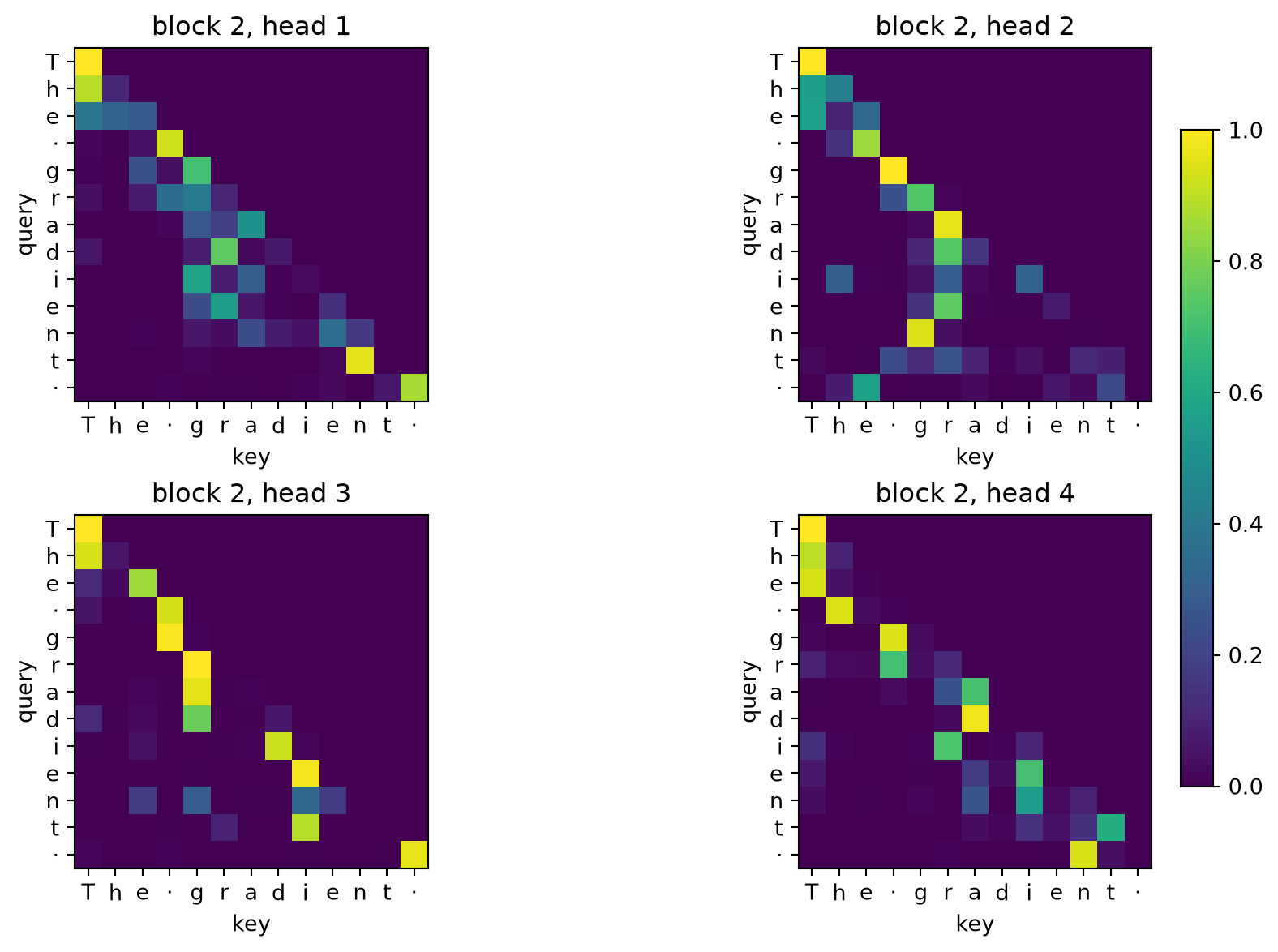

Figure 16.9: Learned attention weights in the second block for the prompt “The gradient ”. The maps are real routing distributions, not explanations or named head roles.

The maps pass both assertions: no future key receives weight and every row sums to one. The heads also differ from one another, but naming one “the previous character head” or another “the word head” from this single prompt would outrun the evidence. Attention shows where values were mixed; the rest of the network can transform, cancel, or ignore what was retrieved.

Listen, but do not grade by fluency

Both Transformer variants can now generate by repeatedly truncating to the most recent 100 characters, predicting a distribution for the next one, sampling, and feeding the result back. Unlike Chapter 12’s LSTM, this simple implementation does not carry a recurrent state; it recomputes the current context on every step.

TipPractice bridge (optional): decoding is another model choice

For next-token logits \(z_i\), temperature is the dial from Chapter 2: it divides each logit by \(T\) before the softmax:

\[ p_i(T)=\frac{\exp(z_i/T)}{\sum_j\exp(z_j/T)},\qquad T>0. \]

Lower \(T\) concentrates probability; higher \(T\) flattens it. Top-\(k\) sampling keeps the \(k\) largest logits, sets the rest to negative infinity, then renormalizes. Nucleus (top-\(p\)) sampling first sorts the model probabilities and keeps the smallest prefix whose cumulative mass reaches \(p\), then renormalizes. The former fixes a candidate count; the latter lets that count adapt to the distribution’s shape. Neither changes the trained weights, and neither guarantees a better sample.

Keeping a set of tokens and renormalizing, as top-\(k\) and nucleus sampling do, is what the causal mask does to each attention row (zero the excluded entries, divide the rest by their sum), with next tokens in place of keys. It gives the distribution over the next token conditioned on that token lying in the kept set. Enforcing a rule that forbids tokens, such as characters that would break the ISO date format of Chapter 13, conditions the distribution at each step in the same way. A sampler that does this at every step need not return the outputs the rule allows in proportion to their probabilities under the model (Exercise 9 of Chapter 13).

For evaluation, if \(L\) is mean token negative log-likelihood in natural-log units, perplexity is \(\exp(L)\). It is an exponentiated loss, not a fluency score. Compare it only under the same tokenization, data, and per-token averaging.

1. Deterministic samples from both Transformer variants.

print("WITH POSITION\n")
# [1]
print(transformer_sample(position_model, "The gradient "))
print("\n\nWITHOUT POSITION\n")
print(transformer_sample(no_position_model, "The gradient "))

WITH POSITION

The gradient choing fine on autograd it by tweight the clue larges of calling functions in What independes the gradients $\rightarrow$ well $\rightarrow$ with nexp for logits collapse it is the stanged
normalized of the argument builds give if the five is the funit or principled update a threshat mactumes at tow


WITHOUT POSITION

The gradient explens ine. The beveuind or clos? we the canlay. Wet orurle
this moples doing ther diest the the contive losio thes despunction erbiveng or of a the
corno isy la prenod in thrathe s to derngexperevive. With the chate is the compfathes bl. Thicte olo
tat ur is $L$\vect{w}^\vect{w} = \mectrimes \vect

The positional sample has the book’s punctuation, fragments of mathematical vocabulary, and stretches that resemble prose. It still loses its argument. The no-position sample is visibly rougher. Neither qualitative judgment replaces the held-out loss; a sample is one stochastic path, while the loss evaluates every held-out target under the model’s full probability distribution.

16.7 What the architecture bought

This comparison covers one small Transformer. It shows what that model gained and what it cost.

Direct content routing. Any earlier visible token can contribute to the next representation in one attention sublayer. The recurrent state no longer has to compress the entire past before the current token can consult it.

Short paths, dense work. The graph distance between visible tokens is short, but the routing matrix is quadratic in context length. Global access is a different tradeoff, not free memory.

Position becomes a modeling choice. Convolution and recurrence bake in local order. Attention asks the designer to supply position and to decide visibility. Chapter 18 will change visibility itself; Chapter 19 will revisit what happens when global routing trades away an image model’s locality bias.

A modular residual stream. Attention moves information, the FFN transforms it, and residual additions let both write into a shared representation. LayerNorm keeps each token’s feature scale manageable along the way.

The causal mask is therefore more than an implementation detail. It says which information a representation is allowed to use: visibility is a modeling decision.

During autoregressive generation, exact softmax attention also turns the past into a memory and compute cost: each new query must read every earlier key and value. A key/value (KV) cache retains each layer’s earlier key and value rows so a new query can reuse them instead of recomputing the whole prefix. In the regression language of Chapter 14, the KV cache is the nonparametric estimator’s dataset: one new query still reads a table that grows with \(t\), but the earlier rows do not have to be rebuilt. Our sampler instead recomputes a cropped 100-character window. A persistent full-prefix cache would retain a different context once that window moves. A cached implementation therefore needs an explicit context and position policy; it is not simply a drop-in acceleration of this sampler. Appendix C separates caching from FlashAttention’s I/O schedule.

What if we keep the regression perspective but change the kernel, the predictor class, or the update rule? The next interlude compares the growing KV cache with a finite sufficient state and a delta update.

Readers who want the diagnostic side of these mechanisms will find kernel geometry, exact I/O-aware algorithms, parallel recurrence, and feature-learning regimes in Shakeri (2026), Beyond This Volume.

NoteCheck yourself

Close the book for one minute and rebuild the Transformer block.

• Without positional signals or a mask, why is self-attention permutation equivariant?
• Which three paths write into the residual stream?
• What changes when a causal mask restricts visibility?

16.8 Okay, so: the Transformer routes, then computes

1. Self-attention reuses Chapter 15’s operator within one sequence. \(Q\), \(K\), and \(V\) all come from \(X\); one learned comparison rule is shared over every permitted query–key pair. Training positions can be evaluated together, while autoregressive generation remains sequential.
2. Without positional signals or a mask, self-attention is permutation equivariant, not invariant. \(\operatorname{SA}(PX)=P\operatorname{SA}(X)\). Sinusoidal clocks supply the sense of order that Chapter 9’s kernels had built in and global routing lacks, and their sine/cosine pairs turn relative shifts into rotations.
3. Multi-head attention is shape discipline. Split \((B,n,d)\to(B,h,n,d_h)\), divide scores by \(\sqrt{d_h}\), form \((B,h,n,n)\) routing weights, concatenate, and project. At fixed \(d\), the four leading projections remain about \(4d^2\) parameters.
4. The causal mask defines visibility. Future scores become negative infinity before softmax. The dense operator still performs quadratic work; the mask does not make the forbidden half computationally disappear.
5. The block alternates routing and computation. Multi-head attention mixes positions, the FFN transforms each position, and both write corrections into Chapter 10’s residual stream. LayerNorm is the same normalization equation over a token’s feature axis.
6. Position wins this seed’s controlled ablation. It lowers held-out loss from 2.3405 to 1.9190. In this run, the LSTM has slightly lower held-out loss than the small Transformer, 1.8881 versus 1.9190. Architecture changes inductive bias; it does not guarantee victory in every data and scale regime.

Sources and further reading

• Vaswani et al., Attention Is All You Need: multi-head attention, sinusoidal position, and the original post-LayerNorm encoder–decoder.
• Su et al., RoFormer: Enhanced Transformer with Rotary Position Embedding: rotates queries and keys so their positional interaction is expressed through relative offset.
• Ba, Kiros, and Hinton, Layer Normalization: normalization within one example and identical train/evaluation computation.
• Zhang and Sennrich, Root Mean Square Layer Normalization: RMSNorm’s scale-only normalization and empirical study.
• Xiong et al., On Layer Normalization in the Transformer Architecture: a qualified comparison of pre- and post-LayerNorm optimization, including pre-LayerNorm training without warmup.
• Dong, Cordonnier, and Loukas, Attention Is Not All You Need: Pure Attention Loses Rank Doubly Exponentially with Depth: without residuals, a stack of attention layers drives the token vectors toward a common row, and MLPs only slow that collapse.
• Geva et al., Transformer Feed-Forward Layers Are Key-Value Memories: empirical evidence behind the associative-memory interpretation of FFNs.
• Haviv et al., Transformer Language Models without Positional Encodings Still Learn Positional Information: causal language models trained without positional encodings come close to models with them in held-out loss and still carry each token’s approximate position, and the authors conjecture that the causal mask supplies it.
• Jain and Wallace, Attention Is Not Explanation: an important limit on reading attention maps as explanations.
• Tsai et al., Transformer Dissection: An Unified Understanding for Transformer’s Attention via the Lens of Kernel: attention written as a kernel smoother, with a comparison of kernel choices that includes a symmetric kernel made by tying the query and key projections.
• Holtzman et al., The Curious Case of Neural Text Degeneration: nucleus sampling and the distinction between likely continuations and useful generation behavior.
• Park et al., Grammar-Aligned Decoding: shows that a sampler that forbids, at each step, every token that cannot lead to a grammatical output can return grammatical outputs at rates not proportional to the model’s probabilities, as in Exercise 9 of Chapter 13.
• Shakeri, Deep Learning: Making It Trainable (2026), “Beyond This Volume”: kernel geometry, exact I/O-aware algorithms, parallel recurrence, and feature-learning regimes.

Exercises

1. (Pencil.) Starting from \(Q'=PQ\), \(K'=PK\), and \(V'=PV\), prove each step of \(\operatorname{SA}(PX)=P\operatorname{SA}(X)\) for self-attention without positional signals or a mask. Then show that mean-pooling the token outputs produces a permutation-invariant sequence representation.
2. (Pencil.) For width \(d=512\) and \(h=8\), write every tensor shape in multi-head attention for \(B=32\) and \(n=100\). Count the weights in \(W_Q,W_K,W_V,W_O\). Repeat for \(h=16\) and explain which dimensions change while the leading parameter count does not.
3. (Code.) Deliberately transpose the causal mask in Figure 16.6, then design an assertion that identifies the first leaked query-key pair. Next set forbidden probabilities to zero after softmax and measure the row-sum error.
4. (Code.) Replace the fixed sinusoidal table with a learned \(\text{Embedding}(100,d)\) while preserving the exact initialization and window schedule protocol. Compare held-out loss. Then extend the sinusoidal buffer by evaluating its formula beyond position 99, and propose an explicit extension rule for the learned table before testing either model on a longer context. Which design has a natural extension, and which has to invent one?
5. (Code.) Aggregate learned attention by relative offset across the held-out tail rather than naming heads from one prompt. Report a distribution for every head and block. Then perturb the highest-weight key’s value vector and measure the logit change. Explain why routing weight and causal influence need not rank tokens identically.

---

1. Tying \(W_Q=W_K\) makes the matrix symmetric and positive semidefinite. In the translation and sequence-prediction experiments of Tsai et al., tying made little difference to performance at the same projection sizes and saved parameters.