Chapter 12 trained a language model: a recurrent network that predicts the next token of one sequence. We now condition that prediction on a second sequence, the source: an encoder processes the source, and a decoder uses the encoder’s final state to generate the target sequence. The architecture is simple, but training and evaluation require several choices: how to handle padding, which previous tokens to supply during training, and how to select a complete output at inference.
The components are not new. In the autoencoder interlude, an encoder compressed a fixed object and a decoder reconstructed it; here both maps are recurrent, and every source detail the decoder uses still crosses one fixed-size context.
Before recurrence, every model we built used a fixed-size contract: 784 pixels in, 10 logits out; \(28 \times 28\) garments in, one verdict out. Many real tasks break that contract on both ends at once: translation maps a sentence of any length to a sentence of some other length, in a different vocabulary. The six design goals of the previous chapter concerned reading a sequence. The sequence-to-sequence setting adds three goals for writing one:
Output of any length. The model decides where the output ends.
Reordering. An output token may depend on input that arrives after it: the year comes last in march 5, 2021 and first in 2021-03-05.
Conditioning on both sides. Each output token depends on the whole input and on every token already written.
The smallest design that meets all three reuses two recurrent machines already built: one that reads a sequence into a state, and the character model that writes one token at a time from a state.
Four earlier ideas return in new roles: the one-hot linear map of Chapter 1 becomes an embedding table; the estimator cases of Section 4.6.1 fix which tokens a loss averages over; the masked update of Chapter 12 becomes the framework’s packed sequences; and the hard max of Chapter 2 returns as greedy decoding, which commits to the most likely token one step at a time. The rules for training and decoding do not depend on recurrence: targets shifted by one token, a token-level log-likelihood, separate loss and input masks, and greedy or beam search carry over to the attention-based decoders of Parts IV and V.
13.1 Two RNNs and a handoff
An encoder reads the source sequence into a context, and a decoder generates the output from that context token by token, feeding each token back in, as the character model did. The encoder may be any network that maps the source to a context. Here both networks are RNNs: the context is the encoder’s final state, the entire input compressed into fixed-size memory, and the decoder starts from that state. The pair is a language model conditioned on the source.
Our laboratory task keeps the core mechanics of translation: date normalization. The source language is human-written dates in several dialects; the target language is ISO 8601:
march 5, 2021        -> 2021-03-05
26 september 2024    -> 2024-09-26
12/15/1950           -> 1950-12-15
The task has variable-length input, a different output alphabet, and long-range structure: the year arrives last in most sources but must be emitted first. Every target has ten characters, so target padding is not tested. A dialect ambiguity gives beam search two readings to rank: numeric dates are written mm/dd/yyyy by 70% of our imaginary writers (the US convention) and dd/mm/yyyy by 30%, and nothing in 03/05/2021 says which.
List the twelve MONTHS and their day counts in DAYS, with February fixed at 28.
Define the reusable make_date helper.
Implement the two date languages, generated on the fly.
Print four pairs and the split overlaps, then build both vocabularies and print their sizes.
import random, torchimport torch.nn as nnimport torch.nn.functional as Fimport matplotlib.pyplot as plttorch.set_num_threads(4) # pinned: results depend on the CPU thread count# [1]MONTHS = ["january", "february", "march", "april", "may", "june", "july","august", "september", "october", "november", "december"]DAYS =dict(zip(MONTHS, [31, 28, 31, 30, 31, 30, 31, 31, 30, 31, 30, 31]))# [2]def make_date(rng: random.Random) ->tuple[str, str]: mo = rng.randrange(12) d = rng.randrange(1, DAYS[MONTHS[mo]] +1) y = rng.randrange(1950, 2026) iso =f"{y:04d}-{mo+1:02d}-{d:02d}" style = rng.random()if style <0.35: src =f"{MONTHS[mo]}{d}, {y}"elif style <0.6: src =f"{d}{MONTHS[mo]}{y}"elif rng.random() <0.7: src =f"{mo+1:02d}/{d:02d}/{y}"# US convention: mm/ddelse: src =f"{d:02d}/{mo+1:02d}/{y}"# EU convention: dd/mmreturn src, isorng = random.Random(6050)pairs, seen_sources = [], set()# [3]whilelen(pairs) <9000: pair = make_date(rng)if pair[0] notin seen_sources: seen_sources.add(pair[0]) pairs.append(pair)train_pairs = pairs[:8000]valid_pairs = pairs[8000:8500]test_pairs = pairs[8500:]# [4]print(*pairs[:4], sep="\n")train_sources = {s for s, _ in train_pairs}valid_sources = {s for s, _ in valid_pairs}test_sources = {s for s, _ in test_pairs}print("exact-source overlaps: "f"train/valid {len(train_sources & valid_sources)}, "f"train/test {len(train_sources & test_sources)}, "f"valid/test {len(valid_sources & test_sources)}")PAD, BOS, EOS =0, 1, 2# special tokens firstSRC =sorted(set("".join(s for s, _ in pairs)))TGT =sorted(set("".join(t for _, t in pairs)))src_stoi = {c: i +3for i, c inenumerate(SRC)}tgt_stoi = {c: i +3for i, c inenumerate(TGT)}tgt_itos = {i: c for c, i in tgt_stoi.items()}V_src, V_tgt =len(SRC) +3, len(TGT) +3print(f"source vocab {V_src}, target vocab {V_tgt}")
The rejection loop is evaluation hygiene: it removes duplicate source strings before the 8,000/500/500 train/validation/test split, so no source string occurs in two splits. We use validation sources for every learning curve and reserve test sources for one final audit after the design is fixed. The same underlying date may appear in another written dialect, which is the structural generalization we want; exact-string memorization is no longer available.
We use three special tokens, the same conventions as a full translation pipeline: <pad> fills the short sequences of a batch out to a rectangle, <bos> is the decoder’s first input, and <eos> ends every target, so the model decides where its output ends by emitting it. A token here is one character; words or subword pieces would change sequence lengths and vocabulary sizes, not the rules for training and decoding.
The character model fed characters in as one-hot vectors; here each token gets a learned vector from nn.Embedding, a table with one trainable row per vocabulary entry. An embedding is exactly a one-hot vector times a weight matrix, computed as a table lookup: the address is hard, the content is learned. Row 17 is fetched by its index, rigidly; the vector in row 17 is trained like any other weight.
The whole architecture is that encode return value: the LSTM’s final \((\vect{h},
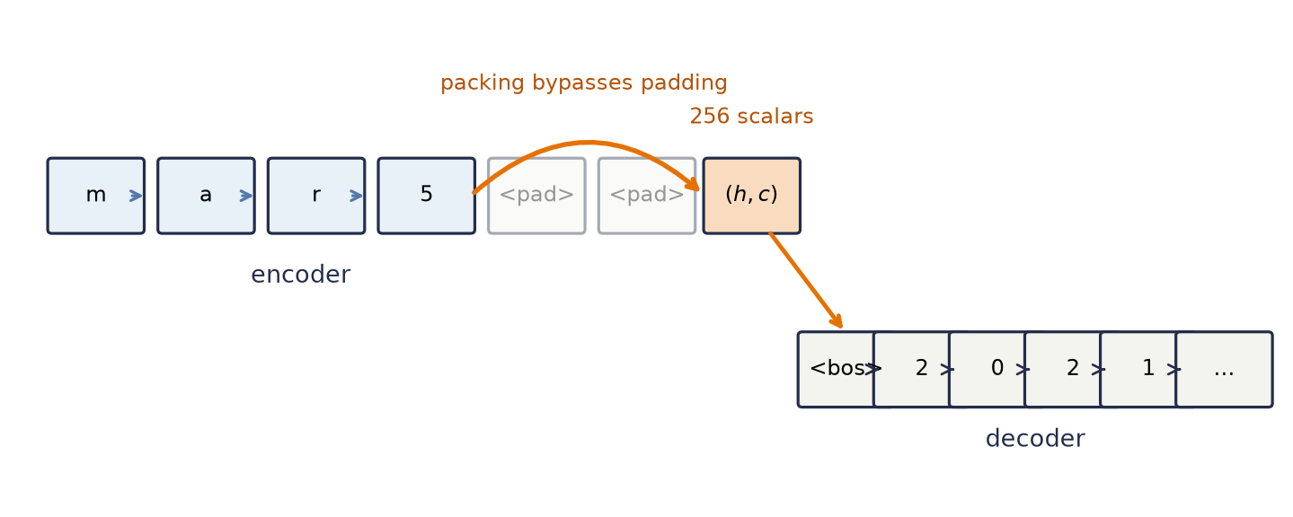
\vect{c})\), handed to the decoder as its initial state. With hidden width 128, that bridge carries two 128-dimensional vectors, or 256 scalars whatever the source length (Figure 13.1). All the source information the decoder can use crosses it.
Figure 13.1: The encoder–decoder handoff. The encoder computes a state at every source position, but only the final \((h,c)\) pair crosses to initialize the decoder; the earlier states are discarded, and packing stops the encoder at the last real token. The decoder feeds each output back as its next input.
13.2 What the loss grades and what the encoder reads
Batching variable-length sequences means padding them to a rectangle. Unless we account for it, padding affects two computations:
The loss. With the mean reduction used here, ignore_index=PAD excludes padded target positions from both the cross-entropy sum and its denominator. Our targets have equal length, so target padding is not tested here. With variable lengths, the calculation is a token mean within each batch; interpreting it as an estimator of corpus-wide token risk also requires specifying how batches are sampled.
The encoder. A zero padding embedding does not make an LSTM update the identity. Processing padded positions can change the final state, making it depend on the padding length as well as the source. Decoding an unpadded sequence can then supply a different context from the one used during training.
The naive model is Seq2Seq with packed=False, so its encoder reads every source to the end of the batch’s padded rectangle. It trains on the same data and budget as the packed model, so the two runs differ only in whether the encoder is told the true lengths (pack_padded_sequence, which runs the recurrence only through each sequence’s real tokens):
Define the reusable helpers: batchify, train_seq2seq, and translate.
Define the reusable helpers: exact_match and unambiguous.
Keep the unambiguous validation and test pairs and list the checkpoint epochs cps.
Train twice: naive right-padding vs. packed sequences.
Print validation exact match on unambiguous dates for the naive and packed models.
# [1]def batchify(prs: list[tuple[str, str]], idx: list[int]) ->tuple[ torch.Tensor, torch.Tensor, torch.Tensor]: srcs = [torch.tensor([src_stoi[c] for c in prs[i][0]]) for i in idx] lengths = torch.tensor([len(s) for s in srcs]) tgts = [torch.tensor([BOS] + [tgt_stoi[c] for c in prs[i][1]] + [EOS])for i in idx] S = nn.utils.rnn.pad_sequence(srcs, batch_first=True, padding_value=PAD) T = nn.utils.rnn.pad_sequence(tgts, batch_first=True, padding_value=PAD)return S, lengths, Tdef train_seq2seq(mode: str="tf", packed: bool=True, epochs: int=25, seed: int=6050, batch: int=128, checkpoints: tuple[int, ...] = ()) ->tuple[ Seq2Seq, dict[int, float] ]: torch.manual_seed(seed) model = Seq2Seq(V_src, V_tgt, packed=packed) opt = torch.optim.Adam(model.parameters(), lr=1e-3) n, curve =len(train_pairs), {}for ep inrange(1, epochs +1): model.train() perm = torch.randperm(n)for i inrange(0, n, batch): S, L, T = batchify(train_pairs, perm[i:i + batch].tolist())if mode =="tf": # ground-truth prefixes: one fused call logits = model(S, L, T[:, :-1])else: # free-running: its own predictions as prefixes state = model.encode(S, L) tok, outs = T[:, :1], []for t inrange(T.shape[1] -1): o, state = model.decoder(model.tgt_emb(tok), state) logit = model.out(o) outs.append(logit) tok = logit.argmax(-1) # feed its own prediction logits = torch.cat(outs, 1) loss = F.cross_entropy(logits.reshape(-1, V_tgt), T[:, 1:].reshape(-1), ignore_index=PAD) opt.zero_grad(); loss.backward() nn.utils.clip_grad_norm_(model.parameters(), 5.0) opt.step()if ep in checkpoints: curve[ep] = exact_match(model, valid_unamb[:400])return model, curve@torch.no_grad()def translate(model: Seq2Seq, src: str, maxlen: int=12) ->str: model.eval() S = torch.tensor([[src_stoi[c] for c in src]]) state = model.encode(S, torch.tensor([len(src)])) tok, out = torch.tensor([[BOS]]), ""for _ inrange(maxlen): o, state = model.decoder(model.tgt_emb(tok), state) tok = model.out(o).argmax(-1) # greedy: best next charif tok.item() == EOS:break out += tgt_itos.get(tok.item(), "?")return out# [2]@torch.no_grad()def exact_match(model: Seq2Seq, prs: list[tuple[str, str]]) ->float:returnsum(translate(model, s) == t for s, t in prs) /len(prs)def unambiguous(prs: list[tuple[str, str]]) ->list[tuple[str, str]]:return [(s, t) for s, t in prsif"/"notin s orint(s[:2]) >12orint(s[3:5]) >12]# [3]valid_unamb = unambiguous(valid_pairs)test_unamb = unambiguous(test_pairs)cps = (2, 4, 6, 8, 12, 16, 20, 25)# [4]naive, _ = train_seq2seq(packed=False)packed, packed_curve = train_seq2seq(packed=True, checkpoints=cps)# [5]print(f"naive right-padding: validation exact match "f"{exact_match(naive, valid_unamb):.1%}")print(f"packed (true lengths): validation exact match "f"{exact_match(packed, valid_unamb):.1%}")
naive right-padding:   validation exact match 37.3%
packed (true lengths): validation exact match 95.7%
Exact match on all unambiguous validation dates is 37.3% for the naive model and 95.7% for the packed one, a 58.4-point gap. The sealed test set remains untouched until we fix both training-mode designs below.
Take the naive model and one short validation source, and watch its encoder state as the input runs past the last real character into the padding:
Append 8 pad tokens to the shortest validation source and record the naive encoder’s states.
Measure encoder-state drift through the padding tail.
# [1]short_src =min((s for s, _ in valid_pairs), key=len)ids = torch.tensor([src_stoi[c] for c in short_src])n_pads =8padded_ids = torch.cat([ids, torch.zeros(n_pads, dtype=torch.long)])with torch.no_grad(): states, _ = naive.encoder(naive.src_emb(padded_ids[None]))states = states.squeeze(0) # (len + n_pads, hidden)T =len(ids)# [2]drift = (states[T -1:] - states[T -1]).norm(dim=1)
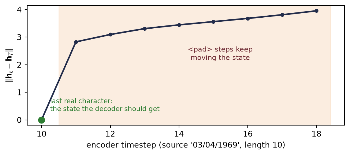
Figure 13.2: Why naive right-padding hurts: the encoder state does not stop when the sentence does. One short validation source is encoded by the naive model; at its last real character (green) the state is exactly what the decoder should receive. A single step already throws the state most of the way to its final drift, and each further step compounds it (navy); the decoder is handed the endpoint of the shaded excursion, a state the unpadded inference-time encoder never produces. Packing simply stops the clock at the last real character.
The masked update of Equation 12.3 keeps the old state on every padded step, so each sequence ends holding the state of its own last real token. pack_padded_sequence is the framework’s version of that bookkeeping: rather than computing the padded steps and throwing them away, it never runs them. If that reading is right, a hand-written masked loop must reproduce the packed encoder’s final states, and the naive encoder must disagree with them for exactly the sources that carried padding.
Write the masked update as a loop over an nn.LSTMCell that shares the encoder’s weights.
Encode 128 validation sources of mixed length three ways with the naive model’s encoder: packed, naive, and masked.
Check that masking reproduces packing and that naive padding moved exactly the padded sources; print the counts.
# [1]@torch.no_grad()def masked_encode(encoder: nn.LSTM, e: torch.Tensor, lengths: torch.Tensor) ->tuple[torch.Tensor, torch.Tensor]: cell = nn.LSTMCell(e.shape[-1], encoder.hidden_size) cell.load_state_dict({k.removesuffix("_l0"): v # same weights, one stepfor k, v in encoder.state_dict().items()}) h = c = torch.zeros(e.shape[0], encoder.hidden_size)for t inrange(e.shape[1]): m = (t < lengths).float()[:, None] # 1 real token, 0 padding h_new, c_new = cell(e[:, t], (h, c)) h, c = m * h_new + (1- m) * h, m * c_new + (1- m) * creturn h, c# [2]S_mix, L_mix, _ = batchify(valid_pairs, list(range(128)))with torch.no_grad(): e = naive.src_emb(S_mix) _, (h_packed, c_packed) = naive.encoder(nn.utils.rnn.pack_padded_sequence( e, L_mix, batch_first=True, enforce_sorted=False)) _, (h_naive, _) = naive.encoder(e)h_masked, c_masked = masked_encode(naive.encoder, e, L_mix)# [3]gap = torch.cat([h_masked - h_packed[0], c_masked - c_packed[0]]).abs().max()assert gap <1e-5moved = (h_naive[0] - h_packed[0]).norm(dim=1) >1e-3padded = L_mix < L_mix.max()assert torch.equal(moved, padded)print(f"{len(L_mix)} validation sources, lengths {int(L_mix.min())} to "f"{int(L_mix.max())}")print("masked update vs packing: same final states (max difference below 1e-5)")print(f"naive padding moved {int(moved.sum())} final states: exactly the sources "f"shorter than {int(L_mix.max())} characters")
128 validation sources, lengths 10 to 18
masked update vs packing: same final states (max difference below 1e-5)
naive padding moved 124 final states: exactly the sources shorter than 18 characters
Packing is the masked update, minus the padded steps it never computes.
WarningTrap: padding is read unless it is masked
Nothing in the tensor marks <pad> as meaningless; meaning is something you enforce, in two places: the loss mask (ignore_index) for the loss, and an input mask (packing, for a recurrent encoder) for the encoder. When a sequence model underperforms unexpectedly, audit both masks before changing the architecture. Telling a model which positions it may not look at is called masking; the loss mask applies the same idea to grading. In a transformer, a causal mask is what turns the model into a language model.
13.3 Teacher forcing: conditioning on target prefixes
Teacher forcing evaluates each observed target token conditional on the source and the preceding target tokens. Summing these negative log-probabilities gives the conditional negative log-likelihood of the observed target sequence. With teacher forcing, the loss in train_seq2seq averages these token losses over the nonpadding target positions of the minibatch.
The two mode branches in the training loop above answer one question. When the decoder is trained, what should it receive as its own previous output?
Free-running (“fr”) feeds the decoder its own most likely token from the step before, as at inference. Early in training those predictions are mostly wrong, so the decoder is trained on prefixes that contain its own errors. Every sequence must also be generated token by token in a Python loop, because step \(t\)’s input does not exist until step \(t-1\) is computed.
Teacher forcing (“tf”) conditions each step on the observed previous token instead. It fixes every decoder input before the forward pass, so the whole target goes through the decoder in one fused decoder call (the model(S, L, T[:, :-1]) line) instead of a Python feedback loop. Whether the positions are then computed one after another or all at once is a property of the decoder, not of teacher forcing: the recurrent decoder still computes each state from the previous one inside that call. From the first epoch, every step is nevertheless conditioned on a correct prefix. The comparison below measures how the two modes differ in validation accuracy during training. The computational difference can be read off the training loop above, one decoder call per batch against one per target position; we do not measure its effect on running time.
Reuse the packed model and its learning curve as the teacher-forced run.
Train the free-running comparison.
Audit all three models once on the final test split.
one final test audit (unambiguous sources):
  naive padding             34.3%
  packed / teacher forced   93.1%
  packed / free-running     99.1%
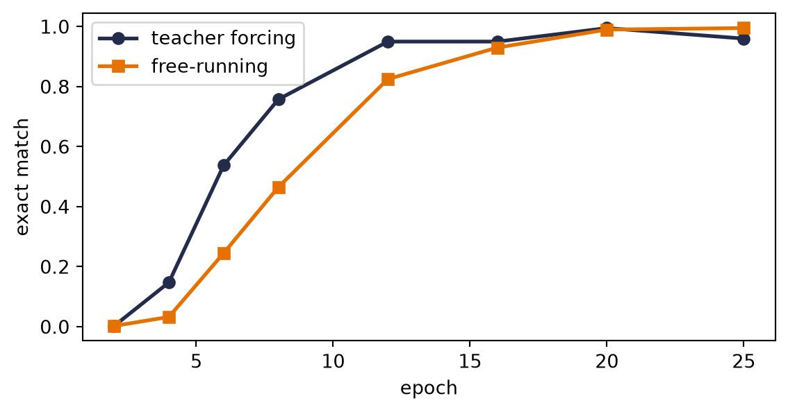
Figure 13.3: Exact match of the two training modes at eight checkpoint epochs, on the first 400 unambiguous validation sources. Teacher forcing leads from epoch 4 through the middle epochs (53.75% vs. 23.75% at epoch 6; 95.00% vs. 81.25% at epoch 12); by epoch 20 the validation curves meet.
On the 400 validation sources of the curves, the teacher-forced model peaks at 99.50% at epoch 20 and ends at 95.75% at epoch 25, so the comparison depends on which checkpoint each model keeps. That choice is part of the design and must be fixed before the test split is opened; here every model is kept as it stands after its last epoch. Free-running, ahead on validation only at the last checkpoint, also finishes ahead in the test audit above; with one seed for each mode, these runs do not show whether that lead would hold on other seeds.
Teacher forcing is the common default, and in this comparison it gained validation accuracy faster early in training. It also creates a mismatch called exposure bias: at inference the decoder conditions on its own predictions, which can form prefixes unlike any seen in training. Exposure bias comes from maximum likelihood on observed prefixes, not from recurrence, so it affects every autoregressive decoder (one that feeds its own outputs back as inputs) trained by teacher forcing. Training never presents the decoder with a prefix that contains its own error, so an early error at inference may also affect the tokens after it. We can look for this effect in the teacher-forced model’s residual errors:
Collect the unambiguous test dates tf_model gets wrong and print how many there are.
Print the first three errors, each beside its truth.
# [1]errs = [(s, t, translate(tf_model, s))for s, t in test_unamb if translate(tf_model, s) != t]print(f"{len(errs)} errors on {len(test_unamb)} unambiguous test dates; a sample:")# [2]for s, t, g in errs[:3]:print(f" {s!r} -> {g!r} (truth {t})")
30 errors on 437 unambiguous test dates; a sample:
  '03/21/1958' -> '1958-03-22'   (truth 1958-03-21)
  '01/22/1996' -> '1996-02-12'   (truth 1996-01-22)
  '21 november 2013' -> '2013-11-22'   (truth 2013-11-21)
The errors are plausible-looking digit substitutions and order slips. The decoder has learned a date-shaped language, but no hard mechanism forces each output field to copy the corresponding source fact. Without the observed prefix, as at inference, one wrong character changes the prefix for every character after it.
NoteScheduled sampling
Scheduled sampling (Bengio et al., 2015) mixes the two training modes. At each timestep, the decoder receives the observed previous token with probability \(\epsilon\) and its own prediction with probability \(1 - \epsilon\), and \(\epsilon\) is annealed from 1 toward 0 as training proceeds. The choice is made per token, not per sequence; committing a whole sequence to model predictions early in training can let consecutive errors amplify. Each step still scores the observed next token, but once some inputs are model predictions, the summed loss is no longer the conditional negative log-likelihood of the observed target. Mixing also has a cost in any architecture: a mixed-in prediction must be generated before it is read, so not all decoder inputs are known before the forward pass. In Exercise 3 you implement it and compare its learning curve with both training modes.
13.4 Getting answers out: search
Given a trained decoder, we want to find the output sequence with the highest probability. That is a search problem over a tree whose nodes branch \(V=V_{\text{tgt}}\) ways; exhaustive search examines \(V^{T}\) sequences, so practical searches walk that tree heuristically.
Greedy search, which translate performs for every exact-match score above, takes the single most probable token at each step and never revises a choice; its cost is \(O(V \cdot T)\). The most probable token at each step need not lead to the most probable sequence, as a tiny decoder shows.
Each row in Table 13.1 is a conditional distribution over the next token; other collects every alternative not named in that row. <eos> ends the sequence.
Table 13.1: A tiny decoder with normalized next-token choices at each listed prefix.
Prefix
Named choice
Alternative
<bos>
A: 0.60
B: 0.40
A
x: 0.55
other: 0.45
B
y: 0.95
other: 0.05
A x
<eos>: 0.80
other: 0.20
B y
<eos>: 0.95
other: 0.05
Greedy chooses A, then x, then <eos>. Multiplying along that path and along the alternative gives
\[
\begin{gathered}
\predictionpart{P(\texttt{A x <eos>})}\\
= \predictionpart{0.60}\times\predictionpart{0.55}\times\predictionpart{0.80}
= \predictionpart{0.264},\\[4pt]
\predictionpart{P(\texttt{B y <eos>})}\\
= \predictionpart{0.40}\times\predictionpart{0.95}\times\predictionpart{0.95}
= \predictionpart{0.361}.
\end{gathered}
\]
The best complete sequence begins with the less likely first token. No hidden continuation overturns this result: the largest probability mass entering an other branch is \(0.60\times0.45=0.27\), and multiplying by further probabilities cannot increase it. This is a specified toy decoder, not a measured model.
Beam search carries the \(k\) best partial sequences (the beam), expands each by all \(V\) tokens and keeps the \(k\) best by cumulative log-probability, at a cost of \(O(k \cdot V \cdot T)\).
In this tree, a beam of width two keeps both A and B. At the next step it keeps B y (0.38) and A x (0.33). Every omitted prefix has probability at most its branch’s total mass (0.27 or 0.02), so none can displace those two. The retained <eos> continuations finish at 0.361 and 0.264. The beam recovers the winner here; a finite beam does not guarantee the best sequence in every tree.
Beam search, k candidate prefixes at once.
# [1]@torch.no_grad()def beam_search(model: Seq2Seq, src: str, k: int=5, maxlen: int=12) ->list[tuple[str, float]]: model.eval() S = torch.tensor([[src_stoi[c] for c in src]]) state = model.encode(S, torch.tensor([len(src)])) beams = [([], 0.0, state, False)] # (tokens, logp, state, done)for _ inrange(maxlen): cand = []for seq, lp, st, done in beams:if done: cand.append((seq, lp, st, True));continue tok = torch.tensor([[seq[-1] if seq else BOS]]) o, st2 = model.decoder(model.tgt_emb(tok), st) logp = F.log_softmax(model.out(o)[0, -1], -1) top = torch.topk(logp, k)for lg, ix inzip(top.values, top.indices): cand.append((seq + [ix.item()], lp + lg.item(), st2, ix.item() == EOS)) beams =sorted(cand, key=lambda b: -b[1])[:k]ifall(b[3] for b in beams):breakreturn [("".join(tgt_itos.get(i, "?") for i in seq if i >2), lp)for seq, lp, _, _ in beams]
Watch the mechanism: winning a step can lose the sequence
If A is the more likely first token, must the most likely complete sequence start with A?
Follow the chapter's fixed probability tree twice. Greedy keeps one continuation; beam width two keeps two partial sequences. Each edge probability belongs to the prefix that reaches it. Node values are their products, including EOS at a completed sequence.
Ask for one answer: choose the best completed candidate. Keeping two candidates does not join their tokens.
0:00 / 0:40
The calculation is readable without playback. Opening this panel loads the optional controls.
The predictor stays fixed; its next-token probabilities depend on the prefix.
Scope and caveats
Blue marks the supplied history, green the model's probabilities. Width counts alternatives at one depth, not tokens generated at once. One requested answer uses the best candidate; the chapter's code keeps the ranked list for inspection. An other stub groups unexpanded alternatives; its mass bounds every completion below it. All such bounds are below this example's winner. EOS contributes to the joint score and stops that sequence. Scores are not renormalized over the beam. Finite-width beam search need not find the global optimum. This picture shows search decisions, not computation time.
Check yourself. Suppose P(x | A) were 0.85 instead of 0.55. Does greedy still miss the best complete sequence?
No. A x EOS becomes 0.60 × 0.85 × 0.80 = 0.408, above 0.361, and every omitted branch is smaller (the largest bound is 0.102). Greedy is not always wrong; it is unguaranteed. It fails when a weaker first step leads to a much stronger continuation.
Transcript and keyboard help
The same fixed tree supports both searches. At its root, A has probability 0.60 and B has probability 0.40. Predict whether winning that first decision guarantees the better complete sequence.
Greedy keeps A and discards B. The discarded branch stays visible with dashed geometry and readable labels; the decoder does not return to it.
After A, greedy chooses x with probability 0.55 rather than the complementary other branch at 0.45. The prefix A x has joint probability 0.330.
After A x, EOS has probability 0.80. The complete joint probability is 0.264. Inspect the discarded counterfactual B y EOS: its three factors give 0.361. The model favored a completion greedy never visited.
Reset the search frontier, not the predictor. Every edge is unchanged. This time allow two partial sequences to remain alive.
The two root candidates A and B both survive, with joint probabilities 0.600 and 0.400. They are two alternatives at depth one, not two consecutive tokens. Width and depth measure different directions in the tree.
Extend each prefix by one token. Blue history A supplies the context for x at 0.55; B supplies the context for y at 0.95. You cannot move that 0.95 to the A branch. The named prefixes B y and A x have joint probabilities 0.380 and 0.330. Every omitted prefix is bounded by its branch's total mass: 0.270 below A, or 0.020 below B. None can displace the two named prefixes. An omitted completion cannot gain probability by adding more conditional factors.
Include EOS and rank the completions: B y EOS scores 0.361; A x EOS scores 0.264. The remaining new other masses are 0.066 and 0.019. All omitted-branch bounds are below 0.361, so the illustrated winner is certified without inventing the omitted subtrees. Both named candidates finish. If we request one answer, choose B y EOS; the chapter's code returns the ranked list so we can inspect alternatives. This success is specific to the fixed example, not a general optimality theorem for beam search. Keep two questions separate: how many alternatives to retain, and how far ahead to compute.
Silent; paused initially; 1.5× playback. Focus the animation pane: Space or K plays/pauses, arrows seek between beats, Home/End jump, Escape pauses. The scrubber and speed menu also work by keyboard. Reduced-motion mode holds each beat's state instead of moving between them.
Search exposes alternatives
An ambiguous date, which the exact-match scores exclude, has two readings, and the generator used the two conventions in the ratio 70/30. Greedy decoding returns one sequence; beam search shows which complete alternatives the model ranks highly:
Keep the slash-format test dates whose first two numbers are both at most 12.
Beam search on genuinely ambiguous dates.
# [1]amb = [(s, t) for s, t in test_pairsif"/"in s andint(s[:2]) <=12andint(s[3:5]) <=12]# [2]for s, t in amb[:4]:print(f"{s!r} truth: {t!r} greedy: {translate(tf_model, s)!r}")for text, lp in beam_search(tf_model, s, k=4)[:2]:print(f" beam: {text!r} joint log score = {lp:.2f}")print()
Each displayed score sums the token log-probabilities along one sequence, including <eos> when it was reached; for a finished sequence it is the log-probability the model assigns to that whole output given the source. These raw joint log scores are log-probabilities of single sequences, not a normalized distribution over the printed beam, so two of them, exponentiated, cannot be read as a 70/30 posterior. The last three dates pair the month/day and day/month readings; the first pairs the month/day reading with 1995-09-20, a hybrid that matches neither convention: beam search searches the model and installs no rule that copies each source field.
For 200 random test dates, ambiguous ones included, we compare the best sequence of a beam of width 5 with the greedy output:
How often beam actually changes the answer.
Print how many of the 200 sampled test dates beam-5 and greedy decode differently.
# [1]sub = random.Random(0).sample(test_pairs, 200)n_diff =sum(beam_search(tf_model, s, k=5)[0][0] != translate(tf_model, s)for s, _ in sub)# [2]print(f"beam-5 disagrees with greedy on {n_diff} of {len(sub)} test dates")
beam-5 disagrees with greedy on 1 of 200 test dates
The two decodings differ once: on this small, well-trained model, beam search changes almost nothing. It became a standard decoder in machine translation, with vocabularies of tens of thousands of tokens and long outputs.
NoteLength normalization
Each token adds a log-probability \(\le 0\) to a raw joint log score, so a raw beam tends to favor short outputs. Dividing each score by \(L^{\alpha}\), with \(L\) the number of scored tokens and \(\alpha\) chosen on validation data, counteracts this; \(\alpha = 1\) ranks by the mean token log-probability. The normalized score is a different decoding objective, which a reported result should name. Every ten-character output has 11 scored tokens (<eos> included), and a common divisor cannot reorder candidates of equal length; in Exercise 4 you inspect the erroneous ones.
13.5 The fixed-size state in the middle
Every source fact the decoder uses crosses one bridge: the encoder’s final \((\vect{h},\vect{c})\) pair, the 256 scalars of Figure 13.1. Our task fits because a date is three facts. The teacher-forced model’s residual digit and order errors are consistent with reconstruction from a compressed summary rather than direct access to source positions; by themselves, they do not prove that compression caused each error. A forty-word sentence would have to cross the same pair, and a wider state may help but gives no direct access to earlier source positions. States for those positions already exist: the encoder computes one at every source position, and this model keeps only the last. A decoder that could consult them at each output step would no longer need one state to carry the whole source.
NoteCheck yourself
Close the book for one minute and reconstruct the sequence pipeline.
Which target positions does the loss grade, which source positions may the encoder read, and what enforces each?
What mismatch does teacher forcing create between training and inference?
What does beam search change, and what part of the learned model does it leave unchanged?
Why does packing leave every final state exactly where the masked update would?
13.6 Okay, so: one training contract, one fixed-size handoff
A sequence-to-sequence model is a conditional language model, here two RNNs and a handoff: <bos> starts the decoder, <eos> lets it choose its length, and embeddings replace one-hots (hard address, learned content).
Padding affects two computations: the loss, where ignore_index removes padded targets from the sum and its denominator, and the encoder, where packing (pack_padded_sequence, the framework’s form of the masked update) keeps padding out of the final state. On the test set, the same model and budget score 34.3% naive versus 93.1% packed. Audit bookkeeping before architecture.
Teacher forcing conditions the decoder on observed prefixes; its token losses sum to the conditional negative log-likelihood of the observed target, and our loop averages them over nonpadding positions. The decoder’s inputs are known in advance, so one fused call replaces the Python feedback loop, but each step still waits for the state of the previous step. Exposure bias is the mismatch between training on observed prefixes and generating from the model’s own. Teacher forcing gained validation accuracy faster early in training; free-running finished ahead on the test set, with one seed per mode and last-epoch checkpoints. Scheduled sampling mixes the two per token, so its decoder inputs are no longer all known before the forward pass.
Decoding is approximate search. Greedy maximizes steps, not sequences, and can miss the highest-probability sequence; beam search carries \(k\) partial sequences for \(O(k V T)\) and surfaces high-scoring alternatives, but a finite beam does not guarantee the best sequence in every tree. Its raw joint log scores are log-probabilities of single sequences, not a posterior over the beam, and a beam can contain invalid hybrids. Length normalization (\(L^{\alpha}\)) changes the decoding objective.
The handoff is the bottleneck. In this model, one fixed-size \((\vect{h},\vect{c})\) pair, 256 scalars, carries all the source information the decoder can use, regardless of input length; the encoder’s per-position states exist and are discarded.
Park et al., Grammar-Aligned Decoding: shows that a sampler that forbids, at each step, every token that cannot lead to a grammatical output can return grammatical outputs at rates not proportional to the model’s probabilities, as in Exercise 9.
(Pencil.) Count this chapter’s parameters: two embeddings, two LSTMs, one output layer, with \(V_{\text{src}} = 37\), \(V_{\text{tgt}} = 14\), embedding size \(e = 32\), and hidden size \(h = 128\). First derive that an LSTM holds \(4\left[(e + h)h + 2h\right]\) parameters (PyTorch keeps two bias vectors). Which components hold most of the parameters, and why is the answer different from Chapter 9’s LeNet audit?
(Pencil.) With vocabulary \(10^4\) and output length 10, compare the number of sequences examined by exhaustive search, greedy, and beam-5. Then explain why beam search with \(k = V^{T}\) is exact and with \(k = 1\) is greedy, why exhaustive search is infeasible at this scale, and why greedy decoding can miss the highest-probability sequence.
(Code.) Implement scheduled sampling: per token, use the observed previous token with probability \(\epsilon\), the model’s own prediction otherwise, annealing \(\epsilon\) linearly \(1 \to 0\) over 25 epochs. Compare its learning curve with both curves in Figure 13.3. Does it inherit teacher forcing’s fast start and free-running’s finish?
(Code.) Add length normalization (\(/L^{\alpha}\)) to beam_search and sweep \(\alpha \in \{0, 0.7, 1\}\) on the date task. Confirm that correct ten-character outputs are unaffected, inspect whether any erroneous beams change, and design the smallest change to the task that would make \(\alpha\) matter.
(Code.) Sutskever et al. (2014) famously improved translation by feeding the source sentence reversed. Try it here. Whatever you observe, explain it with this chapter’s tools: which source-target dependencies does reversal shorten in their setting, and which does it shorten (or lengthen) for dates, where the year sits at the end of the source but the start of the target?
(Code.) Implement BLEU from clipped \(n\)-gram counts and the brevity penalty, then score the ambiguous-date task’s 70/30 output distribution with a fixed seed. Compute corpus BLEU and the mean of sentence BLEU separately, verify the clipped counts on two hand-worked examples, and state which aggregation the evaluation should report. Named wrong answer: “average the sentence BLEUs”: corpus clipping and the brevity penalty do not commute with that mean.
(Code.)Running translator, v2. Keep version 0’s corpus, split, and evaluation (Exercise 6 of Chapter 11), and replace version 1’s slot decoder (Exercise 7 of Chapter 12) with a recurrent decoder that starts from the encoder’s final state. Add <bos> and <eos> to the target vocabulary, pad targets per batch and exclude that padding from the loss with ignore_index, pack or mask the encoder, and train with teacher forcing. Decode the validation split greedily and with a beam of width 5, score both with your BLEU from Exercise 6, and record them in your results log. (Audit.) Break validation BLEU down by source-length bucket for versions 1 and 2. Which version loses more on the longest bucket, and what does the curve say about asking one fixed-size handoff to carry a whole sentence?
(Pencil.)Research bridge (optional). Teacher forcing minimizes per-token cross-entropy on observed prefixes, but the model is judged by a sequence-level score of its own outputs. For a score \(R(\vect{y})\) of an output sampled from \(p_\theta(\cdot\mid\vect{x})\), show that the gradient of \(\E_{\vect{y}}[R(\vect{y})]\) equals \(\E_{\vect{y}}[R(\vect{y})\,\nabla_\theta\log p_\theta(\vect{y}\mid\vect{x})]\), and that subtracting a baseline \(b(\vect{x})\) from \(R\) leaves it unchanged. (Code.) Starting from the teacher-forced date model, fine-tune on sampled outputs with exact match as \(R\) and a running-average baseline, then compare test exact match and the residual errors with the teacher-forced model’s. What did training on its own outputs fix, and what did it cost? The papers listed for this exercise under Sources develop sequence-level training for translation; in Chapter 21 the same gradient returns with a learned reward in place of exact match.
(Pencil.)Forbidding tokens one step at a time. Suppose a rule forbids every token that other collects in Table 13.1, so the allowed outputs are A x <eos> and B y <eos>. A sampler removes the forbidden tokens at each step and renormalizes the rest before it draws. With what probability does it return each allowed output, and which probabilities of Table 13.1 does it replace by 1? Then condition the model’s distribution over complete outputs on the event that the output is allowed: divide each allowed output’s probability by the total probability of the allowed outputs. Which output is more probable under each distribution? State what the per-step sampler guarantees about its output and what it does not. Finally, return to the date task: could a rule that allows only well-formed ISO dates exclude either reading of 03/05/2021? Chapter 16 returns to this per-step rule in its optional practice bridge on decoding.