8  Filters and Convolution (Fixed Kernels)

Chapter tools Lecture 4.1 · Convolutional Neural Networks·Lecture 4.2 · Coding Your First CNN·Download notebook·Open in Colab (opens in a new tab)

As Chapter 6 showed, our fitted MLP was sensitive to small changes in image position. Its dense parameterization imposed neither locality nor weight sharing. After the experimental interlude, we return to these two design choices: restrict a detector to a local patch and apply the same weights at every position.

We first construct this operation with fixed kernels, choosing their coefficients by hand. This lets us inspect what the spatial structure provides independently of training. The convolutional network of Chapter 9 will retain the operation and learn the kernel coefficients from data.

Recall the primitive from Chapter 1: a dot product scores an input against a template. Here the input is a local patch, and the same template is applied throughout the image.

8.1 Two principles, one strategy

The MLP’s failures point to two properties we should build into an image model:

1. Spatial locality. Local neighborhoods contain useful relationships, including edges and textures. A local detector restricts each response to one such neighborhood.
2. Translation equivariance. When an input pattern shifts, the detector’s response should shift with it, wherever the boundary treatment permits the same computation.

These principles suggest a small detector applied to each image patch with the same weights. We begin with hand-designed kernels whose responses are easy to interpret.

8.2 Start in 1D: the moving average

The core operation appears in its friendliest form when smoothing a noisy signal. A moving average replaces each point by the mean of its neighborhood: locality, with uniform weights:

1. Generate a noisy 1D sinusoidal signal and a uniform nine-point averaging kernel.
2. Slide the kernel along the signal with F.conv1d, averaging each nine-point window.

import torch
import torch.nn.functional as F
import matplotlib.pyplot as plt
torch.set_num_threads(4)  # pinned: results depend on the CPU thread count

# [1]
torch.manual_seed(6050)
t = torch.linspace(0, 4 * torch.pi, 300)
noisy = torch.sin(t) + 0.35 * torch.randn(300)
kernel = torch.full((9,), 1 / 9)                       # uniform local weights
# [2]
smooth = F.conv1d(noisy[None, None], kernel[None, None]).squeeze()

We slide a symmetric window along the signal. At each stop, we average the samples under the window and record that mean as the output at the window’s center. The positive and negative fluctuations of the noise largely cancel in the sum, so the rapid jitter is damped while the slow variation of the signal survives. Figure 8.1 shows the operation on a noisy sinusoid; its bottom panel magnifies one nine-point window and the averaging step that produces one point of the smoothed curve.

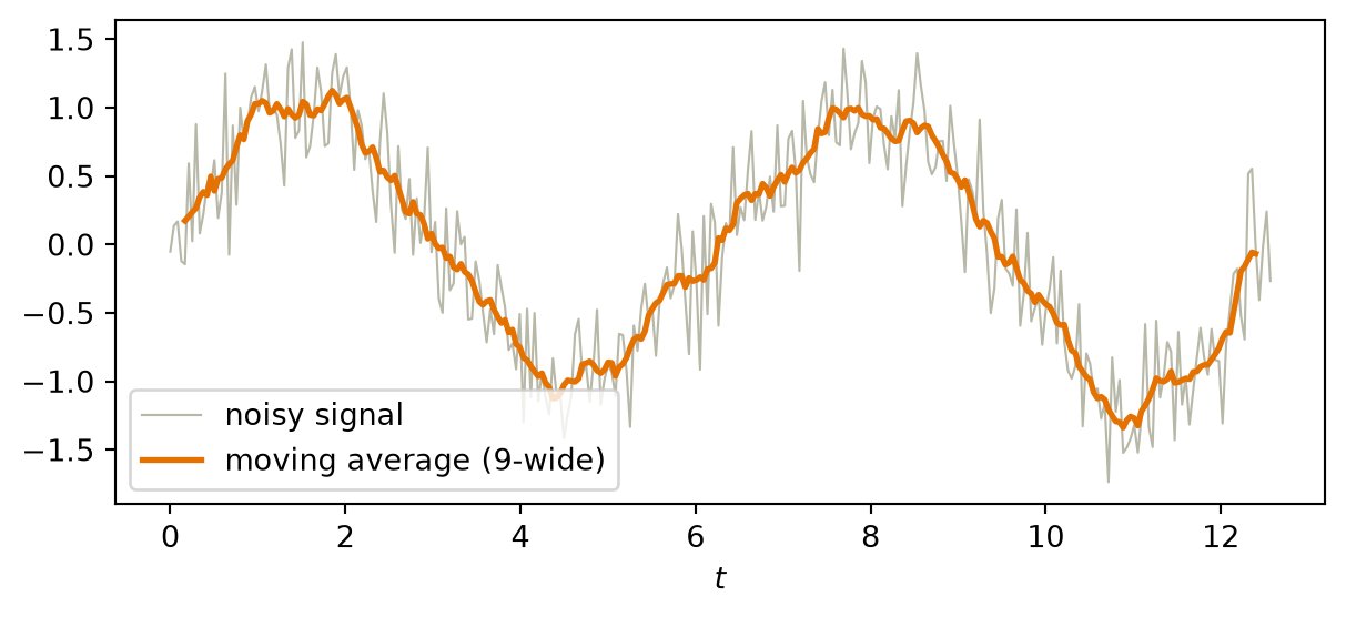
Figure 8.1: A window of uniform weights, slid along a noisy signal, averaging as it goes. Top: the signal, 300 samples of \(\sin t\) on \([0, 4\pi]\) with Gaussian noise of standard deviation 0.35, and its nine-point moving average, computed with F.conv1d; the box marks one window, and the dot on the curve is that window’s output. Bottom: the nine samples in the box, drawn larger as stems from zero, each multiplied by its weight \(1/9\); the nine products sum to the samples’ mean, the output at the window’s center.

Watch the mechanism: one window, one average, then slide

A window nine samples wide slides along the signal, and each average lands at the window's centre. Which samples never get an average of their own?

The moving average from the code above, drawn one window at a time: the same 300 seeded samples, the nine equal weights of torch.full((9,), 1 / 9), and the average each window writes.

\( \predictionpart{y_i} = \class{ba-sum}{\sum_{k=-4}^{4}} \class{ba-weight}{\tfrac{1}{9}}\, \featurepart{x_{i+k}} \)\( \class{ba-count}{300 - 9 + 1 = 292} \text{ averages} \)

Keep the slide, change the nine numbers: every filter in this chapter makes this move.

The calculation is readable without playback. Opening this panel loads the optional controls.

Nothing here is learned or tuned: the nine weights are fixed at one ninth, and the samples are the chapter's own seeded draw.

Scope and caveats

The magnified view above the window is a drawing device, not a second signal: it shows the nine samples the window currently covers at a legible size, with each one shrunk to a ninth and the nine pieces laid end to end, which is what multiplying by the weights and summing does. The samples are the output of the chapter's own cell, seeded with 6050, transcribed at seven decimals; every average is recomputed from them and agrees with the chapter's F.conv1d to better than one part in a million.

Each average is drawn at the centre of its window, which is the convention the chapter's figure uses when it pairs the averages with t[4:-4]. A window nine samples wide fits in 300 − 9 + 1 = 292 places, so the first four and the last four samples are never a centre. Padding the ends would give them averages, at the price of inventing samples outside the signal; the chapter does not pad, and neither does this picture.

Blue is the input signal and green the averages the filter produces. The window and its weights are drawn in neutral ink: they are fixed here, and the book keeps orange for weights that are learned, which begins in the next chapter.

Check yourself. Make the window 25 samples wide. How many averages come out, and what slice of t would the plotting line need?

276, and t[12:-12]. A window 25 samples wide fits in 300 − 25 + 1 = 276 places, and its centre can never sit within 12 samples of either end, so twelve samples at each end have no average of their own. The wider window smooths more and loses more.

Transcript and keyboard help

1. Predict. Three hundred noisy samples lie in a row, and a window nine samples wide covers the first nine. Each average will be drawn at the centre of its window. Which samples will never get one?
2. The weights. A magnified view opens above the window and shows its nine samples as stems. Every stem carries the same weight, one ninth.
3. One average. Each stem shrinks to a ninth of its height, and the nine pieces are laid end to end. Where they end is the average, 0.17, and it lands at the window's centre, the fifth sample.
4. Slide. The window moves one sample to the right, covers a new nine, and stacks them again: 0.20, 0.24, 0.27, 0.35 and 0.39 follow, each at its own centre.
5. The whole signal. The magnified view closes and the window sweeps to the end, repeating the same stack at every position and writing the smooth curve as it goes.
6. Hold. The window has reached the last sample and can go no further. Which samples never got an average?
7. The ends. The first four samples and the last four were never the centre of a window: 300 samples give 300 minus 9 plus 1, that is 292 averages, which is why the chapter plots them against t from index 4 to four before the end.
8. Keep the slide, change the nine numbers. Every filter in the rest of this chapter makes exactly this move with a different set of weights.

Silent; paused initially; 1.5× playback. Focus the animation pane: Space or K plays/pauses, arrows seek between beats, Home/End jump, Escape pauses. The scrubber and speed menu also work by keyboard. Reduced-motion mode holds each beat's finished state instead of moving between them.

8.3 To 2D: the recipe

The moving average extends to images when the window becomes a small square. In two dimensions the weights form a \(k \times k\) array, the kernel, and we slide it across the rows and columns of the image. At each position the kernel covers a \(k \times k\) patch of pixels. We multiply each pixel by the kernel weight that lies over it and sum the \(k^2\) products into one output value.

If we flatten the patch and the kernel into two vectors of length \(k^2\), this sum of products is their dot product: the template score of Chapter 1, applied to one neighborhood of the image. Repeating it at every position where the kernel fits inside the image produces a new two-dimensional array of responses, called a feature map. The operation’s five-step recipe sits beside the three lines that carry it:

1. Define a small window of weights, the kernel (for a blur: all positive, summing to 1).
2. Place the kernel over a patch of the image.
3. Multiply elementwise: kernel weights against the pixels underneath.
4. Sum the products into one output pixel. (Steps 3–4 are one dot product: the patch, scored against a small template.)
5. Slide the window to the next location and repeat, producing a new image.

def manual_conv2d(x: torch.Tensor, k: torch.Tensor) -> torch.Tensor:
    """Cross-correlate an image and kernel over a view of sliding patches."""
    kh, kw = k.shape                               # [1]
    patches = x.unfold(0, kh, 1).unfold(1, kw, 1)  # [2][5]
    return (patches * k).sum(dim=(-1, -2))         # [3][4]

def conv2d(x: torch.Tensor, k: torch.Tensor) -> torch.Tensor:
    return F.conv2d(x[None, None], k[None, None]).squeeze()

torch.manual_seed(6050)
x_test = torch.rand(10, 12)
k_test = torch.randn(3, 3)
gap = (manual_conv2d(x_test, k_test) - conv2d(x_test, k_test)).abs().max()
print(f"recipe vs. torch.conv2d: max |diff| = {gap:.1e}")

recipe vs. torch.conv2d: max |diff| = 4.8e-07

As the markers show, steps 2 and 5 share a line. The plan moves one window at a time, while the code computes every dot product at once: the two unfold calls return all the windows of the image as one view, and the next line scores each window against the kernel. The second function, conv2d, wraps PyTorch’s F.conv2d; the rest of the chapter uses it, and the two functions agree to float32 rounding.¹

The feature map is smaller than the image. We take an odd kernel size, \(k = 2\Delta + 1\), so the kernel has a center entry and reaches \(\Delta\) pixels to each side of it; a \(3 \times 3\) kernel has \(\Delta = 1\). A window that stays inside the frame keeps its center at least \(\Delta\) pixels from every edge, which leaves \(n - 2\Delta = n - k + 1\) positions in each row and each column of an \(n \times n\) image. The output is therefore \((n - k + 1) \times (n - k + 1)\). Padding the image with extra pixels controls this shrinkage, and a stride moves the window in larger steps; Chapter 9 treats both.

Watch the mechanism: one patch, one output

Nine pixels under nine fixed weights: what single number comes out?

An optional walkthrough of Exercise 1. The nine weights are the vertical Sobel edge detector from the examples of fixed filters below, and they stay fixed throughout. Predict where the detector will respond before playing.

PlaceMultiplySumSlide

Input · 4 × 4

0011 0011 0011 0011

Fixed kernel: vertical Sobel · 3 × 3

−101 −202 −101

Multiply matching entries

001 002 001

Output · 2 × 2

4444

0 + 0 + 1 + 0 + 0 + 2 + 0 + 0 + 1 = 4

Every valid patch crosses the edge. The same fixed kernel produces 4 at each of the four output positions.

One-pixel steps, no padding, no kernel flip, and no learning. An unwritten output is shown as “·”, not zero.

Check yourself. Keep this 3 × 3 kernel but give it a 6 × 6 image. How many output values does the valid convolution produce?

Sixteen. The patch fits in 6 − 3 + 1 = 4 places along each axis, so the output is 4 × 4. Here 4 − 3 + 1 = 2 gave the 2 × 2 map you watched being filled.

Read the walkthrough

1. Place. Start with the top-left 3 × 3 patch. Each row is (0, 0, 1). The input is blue; the hand-chosen kernel is neutral.
2. Multiply. The rays trace the top-right pixel of the patch and the top-right kernel weight into a multiplication point: 1 × 1 = 1. Its outgoing ray reaches the top-right product. Apply the same rule at all nine matching positions. The three product rows are (0, 0, 1), (0, 0, 2), and (0, 0, 1).
3. Sum. Nine rays bring all nine products, including zeros, to one addition point. Their sum is 1 + 2 + 1 = 4. The outgoing green ray writes that value into the top-left output cell.
4. Slide. Move right, then down, then left. These visits fill the other three output cells. The weights never change. Each valid patch crosses the same vertical edge, so every sum is 4.

Keyboard: focus the animation pane and use Space to play or pause, Left/Right to step, Home to return to the start, or End to reach the end. The animation is silent, with on-screen explanations.

The animation is a compact adaptation of the accompanying convolution demonstration. Its order is sequential; the unfold implementation above scores all patches together.

8.4 Examples of fixed filters

The sliding dot product stays the same. Changing the kernel weights changes what it detects. We apply three classic kinds of kernel to a synthetic test scene and to a boot from our Fashion-MNIST subset:

• Blur uses uniform positive weights summing to 1, the 2-D moving average.
• Sharpen amplifies each pixel’s difference from its neighbors.
• Edge detection (Sobel) uses positive and negative weights summing to zero. Over any flat region the products cancel and the output is silent; over an edge, a sharp change in values, the sum swings large. Its response at each position indicates whether intensity changes there along the kernel’s direction.

Watch the mechanism: why the Sobel kernel responds to one edge and not the other

The rectangle's left side and its top are both edges, where the image jumps from dark to bright. Which one does the vertical Sobel kernel see?

The zoo's vertical Sobel kernel, taken apart before the code below uses it: nine numbers read as two operations, sliding over the top-left corner of the rectangle that make_shapes draws.

\( \begin{bmatrix} -1 & 0 & 1\\ -2 & 0 & 2\\ -1 & 0 & 1 \end{bmatrix} = \class{sb-along}{\begin{bmatrix} 1\\ 2\\ 1 \end{bmatrix}}\,\class{sb-across}{\begin{bmatrix} -1 & 0 & 1 \end{bmatrix}} \)\( \predictionpart{h} = \class{sb-along}{1}\,d_1 + \class{sb-along}{2}\,d_2 + \class{sb-along}{1}\,d_3, \quad \class{sb-across}{d_r = \featurepart{x}_{r,\text{right}} - \featurepart{x}_{r,\text{left}}} \)

Average along the edge, difference across it: that is a vertical-edge detector.

The calculation is readable without playback. Opening this panel loads the optional controls.

This is the kernel's arithmetic on one corner of the chapter's synthetic scene: nothing is learned, and the boot and the other four kernels are left to the code below.

Scope and caveats

The kernel is exactly the product of a column and a row: the column (1, 2, 1) averages three neighbouring rows with the middle one counted twice, which is the moving average from the start of the chapter with uneven weights, and the row (−1, 0, 1) subtracts the left pixel from the right one and ignores the middle. Multiplying the two gives the nine numbers in the code, so sliding the kernel is the same as taking a difference across each row and averaging those differences down the column.

The picture is an eight-by-eight crop of make_shapes(), rows 7 to 14 and columns 5 to 12, where every pixel is either 0 or the rectangle's 0.9. Each response is drawn at the centre of the patch that produced it; the code's valid convolution returns the same numbers one pixel in from every edge, which is why its output is 62 by 62 for a 64 by 64 scene. Nothing here is interpolated: every value is recomputed from the declared kernel and the rectangle, and agrees with torch's conv2d on the full scene.

On the rectangle's right side, where the image falls from 0.9 to 0, the same kernel gives −3.6: the same size, the opposite sign, which is why that side prints dark and the left side bright in the zoo's gray panels. Blue is the input image, green the kernel's response, and the kernel itself is drawn in neutral ink because it is fixed; the book keeps orange for weights that are learned, which begins in the next chapter.

Check yourself. The zoo's other Sobel kernel, [[−1, −2, −1], [0, 0, 0], [1, 2, 1]], is this one transposed. What does it give on this corner's top edge, and on its left side?

3.6 on the top edge and 0 on the left side. Transposed, the kernel takes its difference down each column, bottom minus top, and averages the columns 1, 2, 1: along the top every column climbs by 0.9, while on the left side each column is flat. Transposing swaps which edges the kernel sees.

Transcript and keyboard help

1. Predict. An eight-by-eight corner of the chapter's rectangle: dark pixels of 0 above and to the left, bright pixels of 0.9 below and to the right. The left side and the top are both edges. Which will the vertical Sobel kernel see?
2. Two jobs. The nine numbers are a column times a row. Across each row the kernel takes the right pixel minus the left one, ignoring the middle; down the rows it averages those differences with weights 1, 2 and 1.
3. A flat patch. Inside the rectangle every pixel under the frame is 0.9, so every row's difference is 0 and the response is 0: bright, but silent.
4. The left side. The frame slides onto the rectangle's left side. In every row the right pixel is 0.9 and the left one 0, so each difference is 0.9; weighted 1, 2 and 1 they add up to 3.6.
5. Hold. The frame moves onto the top edge, dark above and bright below. The image changes just as sharply here. Predict the response.
6. The top. Each row under the frame is flat, the dark row and the two bright rows alike, so every difference is 0 and the response is 0. The change runs down the rows, and this kernel compares only across them.
7. Everywhere. The frame visits every position and leaves its response behind: a stripe down the left side, 0.9, 2.7 and then 3.6 once the frame is fully inside the rectangle's rows, and nothing along the top.
8. The lesson. An average along the edge and a difference across it make a vertical-edge detector; the code below applies the same nine numbers, and their transpose, to the whole scene and to a boot.

Silent; paused initially; 1.5× playback. Focus the animation pane: Space or K plays/pauses, arrows seek between beats, Home/End jump, Escape pauses. The scrubber and speed menu also work by keyboard. Reduced-motion mode holds each beat's finished state instead of moving between them.

1. Define the reusable make_shapes helper.
2. Load one boot image and define five 3×3 kernels: identity, blur, sharpen, and two Sobel edge detectors.
3. Draw each kernel’s nine weights, all five on one shared scale centered at zero.
4. Apply every kernel to both images and show the outputs.

# [1]
def make_shapes(n: int = 64) -> torch.Tensor:
    img = torch.zeros(n, n)
    img[10:26, 8:30] = 0.9                                   # rectangle
    yy, xx = torch.meshgrid(torch.arange(n), torch.arange(n), indexing="ij")
    img[((yy - 44) ** 2 + (xx - 20) ** 2) < 100] = 0.6       # disk
    stripes = ((xx + yy) % 12 < 5).float() * 0.8
    img[8:56, 40:60] = stripes[8:56, 40:60]                  # diagonal stripes
    return img

# [2]
development = torch.load("../../data/fashion-train.pt")
boot = development["X"][(development["y"] == 9).nonzero()[0, 0]].float() / 255.0

kernels = {
    "identity": torch.tensor([[0., 0., 0.], [0., 1., 0.], [0., 0., 0.]]),
    "blur": torch.full((3, 3), 1 / 9),
    "sharpen": torch.tensor([[0., -1., 0.], [-1., 5., -1.], [0., -1., 0.]]),
    "Sobel (vert.)": torch.tensor([[-1., 0., 1.], [-2., 0., 2.], [-1., 0., 1.]]),
    "Sobel (horiz.)": torch.tensor([[-1., -2., -1.], [0., 0., 0.], [1., 2., 1.]]),
}

from fractions import Fraction
from matplotlib.colors import LinearSegmentedColormap

fig, axes = plt.subplots(3, 5, figsize=(7.8, 5.0))
# [3]
signed = LinearSegmentedColormap.from_list("signed", ["#4A5566", "white", "#6F6152"])
scale = max(k.abs().max().item() for k in kernels.values())   # shared by all five
for col, (name, k) in enumerate(kernels.items()):
    axes[0, col].imshow(k, cmap=signed, vmin=-scale, vmax=scale)
    for i in range(3):
        for j in range(3):
            w = k[i, j].item()
            label = str(Fraction(w).limit_denominator(9)).replace("-", "\u2212")
            axes[0, col].text(j, i, label, ha="center", va="center", fontsize=8,
                              color="white" if abs(w) > 0.6 * scale else "#232D4B")
    axes[0, col].set_title(name, fontsize=9)
# [4]
for row, image in enumerate([make_shapes(), boot], start=1):
    for col, (name, k) in enumerate(kernels.items()):
        axes[row, col].imshow(conv2d(image, k), cmap="gray")
for ax in axes.flat:
    ax.set_xticks([]); ax.set_yticks([])
plt.tight_layout(); plt.show()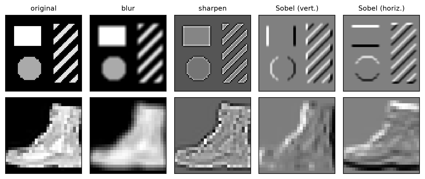

Figure 8.2: One operation, five kernels. The top row prints the nine weights of each 3×3 kernel (identity, blur, sharpen, and two Sobel edge detectors), shaded on one scale centered at zero; each column below applies that kernel to the same two inputs. The middle row is the synthetic scene (\(64 \times 64\), zero except for a rectangle, a disk and diagonal stripes of intensities 0.9, 0.6 and 0.8); the bottom row is the first ankle boot among the development images, scaled to \([0, 1]\). The vertical-edge kernel responds strongly to vertical boundaries, the horizontal one to horizontal boundaries.

Study the two Sobel columns for a moment. The vertical-edge detector lights up on the rectangle’s sides and stays silent on its top and bottom; the horizontal detector does the reverse; the diagonal stripes excite both. With nine numbers we have built a primitive feature detector, the patch-by-patch detector that the two principles suggest, and none of its coefficients was learned.

8.5 Naming the operation

This sliding sum of products is called cross-correlation. To write it down, we index the kernel \(V\) by offsets from its center: the entry \([V]_{u,v}\) sits \(u\) rows and \(v\) columns from the center, with \(u\) and \(v\) running from \(-\Delta\) to \(\Delta\); negative \(u\) lies above the center and negative \(v\) to its left, so in a \(3 \times 3\) kernel \([V]_{-1,-1}\) is the top-left entry. With the kernel centered on pixel \((i, j)\) of the image \(X\), the entry \([V]_{u,v}\) lies over the pixel \([X]_{i+u,\,j+v}\), and the output \([H]_{i,j}\) sums these products over the window:

\[ [H]_{i,j} \;=\; \sum_{u=-\Delta}^{\Delta}\;\sum_{v=-\Delta}^{\Delta} [V]_{u,v}\,[X]_{i+u,\,j+v} . \tag{8.1}\]

This is the sliding dot product written entry by entry, for each center \((i, j)\) at least \(\Delta\) pixels from the edges.

NoteWhy we call it “convolution”

In deep learning, this cross-correlation operation is commonly called a convolution, and we follow that convention. Mathematical convolution flips the kernel before applying it. For a fixed kernel, the flip can change the output, as Exercise 4 demonstrates. For an unrestricted learned kernel, it amounts to a reparameterization of the same family of operations.

8.6 Translation equivariance

Unlike the dense layer of Chapter 6, cross-correlation applies the same kernel at every position. On the interior of the image, shifting the input therefore shifts the feature map by the same displacement and leaves its values unchanged. This property is translation equivariance.

We test it as a question of order: does shifting before filtering give the same result as filtering before shifting?

1. Filter the shifted image, and shift the filtered image, with the vertical Sobel kernel.
2. Compare the two orders on the interior, away from the blank border.

# [1]
img = make_shapes()
sobel = kernels["Sobel (vert.)"]
s = 5

shifted = torch.zeros_like(img)
shifted[:, s:] = img[:, :-s]                  # input shifted right by 5

A = conv2d(shifted, sobel)                    # filter the shifted image
B = conv2d(img, sobel)                        # filter, THEN shift the result
B_shifted = torch.zeros_like(B)
B_shifted[:, s:] = B[:, :-s]

interior = (A - B_shifted)[:, s + 2:]         # compare away from the blank border
# [2]
print(f"filter(shift(x)) vs shift(filter(x)): max |diff| = {interior.abs().max():.1f}")

filter(shift(x)) vs shift(filter(x)): max |diff| = 0.0

With the scene shifted \(s = 5\) pixels to the right, the difference prints as 0.0 away from the left edge, in all but the first \(s + 2\) output columns (the \(s\) columns that read the zero fill, plus a margin of two). The detector’s response moves with the scene.

The contrast with Chapter 6 is structural. A dense layer gives every input pixel its own coefficient in every output, so its weights are tied to absolute positions in the frame. Cross-correlation ties its weights to offsets from the window’s center, so a pattern produces the same response wherever it appears. Near the edges the equality can fail, because a window there covers pixels that the shift filled with zeros or pushed out of the frame; exact equivariance holds on the interior, which is why the code excludes the border columns.

Before going further, keep two related properties distinct:

• Equivariant means that the output transforms along with the input: if the input moves, the feature map moves by the same displacement. Convolution provides this.
• Invariant means that the output does not change at all: a garment classifier should predict the same category wherever the garment sits in the image.

Equivariance tracks where a feature is; classification needs invariance, because the label depends on what is present. Equivariance is the raw material for invariance. In Chapter 9, pooling discards some position information to gain local shift tolerance, and Chapter 10 pools each feature map over the whole image. Edge effects, strides and pooling windows can still change intermediate responses under a shift, so whether a whole network is shift invariant must be measured at its output, not presumed.

8.7 The matrix view: a structured, weight-shared linear map

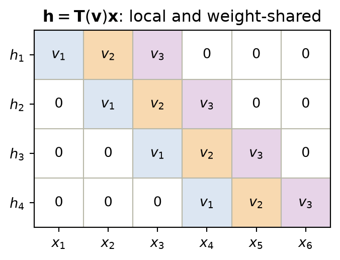
Every output is a dot product of a few inputs with the kernel weights, so cross-correlation is a linear map: it can be written as one matrix multiplying the flattened input. We build that matrix in Figure 8.3 for a one-dimensional signal of six inputs and a kernel of three weights \(v_1, v_2, v_3\), which gives four outputs. Each row of the matrix is one position of the window. Row 2 computes \(h_2 = v_1x_2 + v_2x_3 + v_3x_4\): it holds the three weights in the columns of the inputs under its window and zeros everywhere else. With \(v_1 = v_2 = v_3 = 1/3\), the matrix computes a three-point moving average.

The matrix has two kinds of structure. Half its entries are zero here, and nearly all of them for an image, because each output depends only on its window (locality). The nonzero entries repeat, because every row holds the same three weights, one column further right than the row above (weight sharing). A dense \(4 \times 6\) matrix has 24 independent entries; this one has 3.

The saving grows with the input. A dense layer from our 28×28 images to an equal-sized output (with padding) would have \(784 \times 784 \approx 615{,}000\) weights; the Sobel detector has nine, reused at every position. These are the constraints of Chapter 6 made concrete: locality zeroes out most of the matrix, weight sharing ties the remaining entries together, and what is left is a linear map with almost nothing to specify.

1. Construct the sparse weight-shared matrix.

from matplotlib.colors import ListedColormap

# [1]
weight_ids = torch.zeros(4, 6)
for row in range(4):
    weight_ids[row, row:row + 3] = torch.tensor([1, 2, 3])

Figure 8.3: One-dimensional cross-correlation written as a matrix, for six inputs, a kernel of three weights and four outputs. Each row is one position of the window, with \(v_1, v_2, v_3\) in the columns of its three inputs and zeros elsewhere. A 2-D image gives the analogous block-structured matrix.

8.8 The bottleneck: someone has to design the kernel

Why did this classical machinery not solve vision decades ago? The kernels are only as good as their designers, and hand-crafted kernels have three limitations:

1. Predefined features. These kernels were selected for specific low-level operations, such as smoothing or detecting intensity changes, rather than fitted to the classification task.
2. Manual feature engineering. Choosing which kernels to use, and how to combine them, takes deep domain expertise and extensive experimentation for every new task.
3. No adaptation. A fixed kernel cannot adjust to a dataset. What works for one task fails for another.

An entire era of computer vision operated under these constraints, chaining hand-engineered filters into multi-stage heuristic pipelines. The architectural geometry (local receptive fields with shared spatial weights) was sound; the manually tuned coefficients formed the bottleneck.

A \(3 \times 3\) kernel contains nine scalar coefficients. We can treat them as a parameter tensor \(\matr{V} \in \mathbb{R}^{3 \times 3}\) and optimize a task loss using the gradients from Chapter 5. Locality and weight sharing remain fixed; the coefficients become learnable. This gives a trainable convolutional layer. Chapter 9 combines such layers into a classifier.

NoteCheck yourself

Close the book for one minute and reconstruct the sliding operation.

• Which two design commitments create locality and translation equivariance?
• Why does weight sharing turn a dense linear map into a small kernel?
• What remains hand designed at the end of this chapter?

8.9 Okay, so: the machine before the learning

1. One operation, many kernels: slide a small template, take a dot product at every position (Equation 8.1). Blur, sharpen, and edge detection differ only in the kernel’s numbers.
2. Locality and sharing are built in: as a matrix, convolution is almost-all-zero with nine numbers repeating: 615,000 weights collapsed to 9.
3. Equivariance is exact on the interior, not approximate: filter-then-shift equals shift-then-filter wherever both operations use the same pixels. Boundary handling must be specified separately. Pooling in Chapter 9 adds some local shift tolerance on top of that equivariance.
4. Hand-crafting is the bottleneck: predefined features, engineering cost, no adaptation. Gradient descent can learn the kernel’s numbers instead.

Sources and further reading

• Fukushima, “Neocognitron: A Self-organizing Neural Network Model” (1980): an early hierarchy of local, shift-tolerant feature detectors.
• LeCun et al., “Gradient-Based Learning Applied to Document Recognition” (1998): connects shared local kernels to the trainable CNN built next.
• Dumoulin and Visin, “A Guide to Convolution Arithmetic for Deep Learning” (2016): a visual reference for padding, stride, and output-shape arithmetic.
• PyTorch’s documentation for Tensor.unfold specifies the sliding-window view that manual_conv2d scores against the kernel.

Exercises

1. (Pencil.) Compute by hand the full output of cross-correlating with the vertical Sobel kernel the \(4\times4\) image whose rows are all \((0,0,1,1)\). Before computing: where should the detector fire?
2. (Pencil.) (a) Design a \(3\times3\) kernel that detects diagonal edges (bottom-left to top-right). State your design rule: what must the weights sum to, and why? (Code.) (b) Run it on make_shapes() and check that it fires on the stripes.
3. (Pencil.) Prove translation equivariance from Equation 8.1: substitute the shifted image \(X'_{i,j} = X_{i-s,j}\) and show \(H'_{i,j} = H_{i-s,j}\). Why does the same argument fail for the MLP of Chapter 6? State where the proof applies at a finite image boundary.
4. (Code.) True convolution flips the kernel: run conv2d with k and with k.flip(0, 1) for the blur and for Sobel. Which outputs differ, which do not, and what property of the kernel decides it?
5. (Code.) The box blur is separable: show that convolving with the \(3\times3\) uniform kernel equals convolving with a \(3\times1\) column of \(\tfrac13\)s and then a \(1\times3\) row of \(\tfrac13\)s. Count multiplications per output pixel for each route. This trick mattered in the hand-crafted era.

---

1. A vectorized rewrite of a sliding loop is easy to get wrong by one index or one axis, so we check it against the framework before relying on it. On a random \(10 \times 12\) image and a random \(3 \times 3\) kernel, the largest absolute difference between the outputs of manual_conv2d and conv2d is \(4.8 \times 10^{-7}\), the size of float32 rounding.