Chapter 16 warned that global routing trades away locality bias. Chapter 18 added two pieces: a learned summary token can gather a sequence for a downstream head, and pretraining is a regime, not an architecture. A Transformer reads vectors in a sequence. How do we turn a photograph into such a sequence?
Cut the image into patches, project each patch to a vector, and let the Transformer encoder read those vectors as tokens. That minimalist transplant is the Vision Transformer (ViT). A convolutional network arrives knowing that nearby pixels belong together and that one local detector should slide across the image. ViT arrives knowing much less about images. Which learner wins therefore depends not just on architecture, but on data, training, and scale.
The word scale has two meanings in this chapter. First it means making an image model deeper, wider, or higher-resolution. Then it means fitting empirical laws that connect loss to parameters, tokens, and training compute. The bridge between the two meanings is resource allocation: what should we enlarge, and what must grow with it?
19.1 Let the image become a sequence
Start with the arithmetic used by the original ViT. A color image is \(224\times224\) pixels, and each square patch is \(16\times16\). There are
patches. Each patch contains \(16\times16\times3=768\) raw channel values. So one image has become a sequence of 196 vectors, each initially 768-dimensional, already the same width used by the base Transformer in that paper.
where \(B\) is batch size, \(C\) channels, and \(H,W\) are spatial dimensions. For a square patch width \(P\) that divides both \(H\) and \(W\), the patch count is
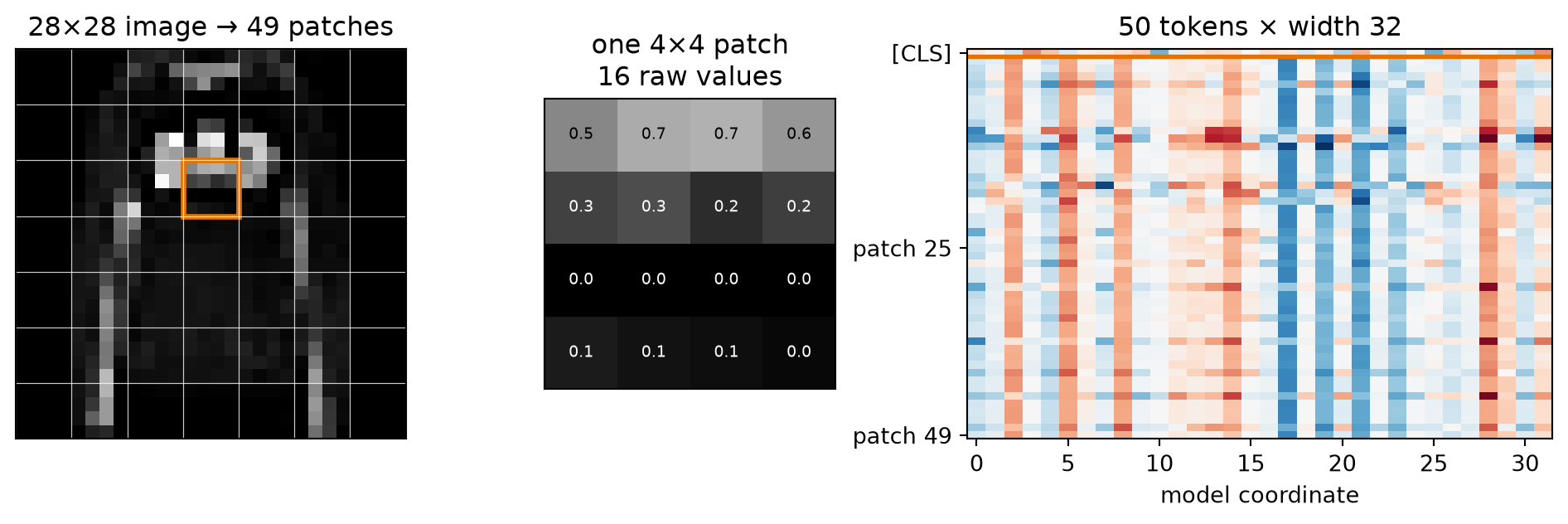
We can see this on the fixed Fashion-MNIST subset first opened in Chapter 6. The \(28\times28\) grayscale images divide into \(7\times7=49\) patches when \(P=4\).
Fix the seed, load 1,200 development and 600 holdout Fashion-MNIST images, and split off 200 for validation.
Load imports, the fixed Chapter 6 split, and image shapes.
projects every raw patch to model width \(d\). The operation has a useful exact identity. Unfold the image, multiply each flattened patch by \(\matr{E}\), and add a bias, or reshape the columns of \(\matr{E}\) into \(d\) convolutional kernels with kernel size \(P\) and stride \(P\). The two computations are the same affine map.
Project one image’s 4×4 patches through F.unfold and a random matrix, and through F.conv2d, then assert they match.
Patchify and verify unfold-plus-linear equals one strided convolution.
raw patches: (1, 49, 16)
projected tokens: (1, 49, 32)
max |linear - convolution|: 7.15e-07
Figure 19.1: An image becomes a sequence. A 28×28 garment is divided into 49 nonoverlapping 4×4 patches (left); one patch contains 16 raw values (center); a shared linear projection maps every patch to width 32, and a separate learned [CLS] row is prepended (right). The displayed projection is random arithmetic, not a trained representation.
The identity means that ViT’s patch projection is a learned, shared local operator, so some image structure survives at the input. What changes is what happens next: instead of stacking local feature maps, we hand the patch sequence to global self-attention.
TipPatchify once, audit twice
Check that \(P\) divides both spatial dimensions, assert the patch and token shapes, and compare unfold-plus-linear with the equivalent convolution to numerical roundoff. Patchification silently changes sequence length, feature width, and the attention cost; one shape mistake propagates through the entire model.
19.2 A sequence-level representation of the patches
The projected patches still need two additions. First, prepend a learned vector \(\vect{x}_{\mathrm{CLS}}\in\mathbb{R}^{d}\). Second, add one learned position vector to every sequence slot. For image \(b\), ViT’s complete encoder input is
Here \(\matr{X}_{\text{patch}}^{(b)}\in\mathbb{R}^{N\times CP^2}\) holds the flattened patches of image \(b\) as rows, \(\matr{E}\in\mathbb{R}^{CP^2\times d}\) is the shared patch projection, \(\vect{b}_{\text{patch}}\in\mathbb{R}^{d}\) is the patch bias shared across patches, \(\mathbf{1}_N\in\mathbb{R}^{N}\) is the all-ones vector, and \(\matr{E}_{\mathrm{pos}}\in\mathbb{R}^{(N+1)\times d}\) contains learned absolute position vectors. The [CLS] row remains separate: it receives neither the patch projection nor the patch bias.
[CLS] does not start as a summary. As in Chapter 18, it supplies a sequence-level representation, and training on the downstream loss determines what its final hidden state carries. Every encoder layer lets that row query the patch rows; after the final layer, a linear head reads its \(d\) coordinates and produces class logits. The original ViT appendix found that class-token and global-average-pooling heads worked similarly after tuning their learning rates. [CLS] is a useful interface, not proof of a superior pooling rule.
Position is essential for a different reason. Without positional information, self-attention is permutation-equivariant: permuting patch rows produces the same permutation of output rows. A symmetric pooling rule can consequently become invariant to patch order, unable to distinguish a sleeve above a shoe from a shoe above a sleeve. Learned positions break that symmetry. In the original ablation, removing position hurt, while learned 1-D, learned 2-D, and relative alternatives performed similarly in that setting. The result supports supplying geometry; it does not establish one universal positional scheme.
ViT then reuses Chapter 16’s pre-LayerNorm encoder block. With \(\matr{Z}_{\ell-1}\in\mathbb{R}^{B\times(N+1)\times d}\),
The residual stream, LayerNorm axis, multi-head routing, and position-wise MLP are unchanged. This is an encoder-only classifier, so there is no causal mask and no decoder. Pre-LayerNorm gives gradients a cleaner residual path; it does not make optimization automatic. The original ViT training recipe still used learning-rate warmup.
19.3 Locality: built in or learned
Chapter 6 called constraints a form of knowledge. Convolution trades flexibility for locality and, at stride one under matched boundary conditions, for translation equivariance; ViT gives up much of that image-specific prior, so useful geometry must come from data, optimization, or a new architectural constraint.
Convolutional network
Vision Transformer
Local, spatially shared kernels
Content-dependent routes between all patch tokens
Spatial sharing; stride-one convolution is equivariant under the stated boundary conditions
Geometry supplied mainly by patches and position vectors
Global sight accumulated through depth
Every patch reachable in one attention layer
Strong image-specific prior
More freedom, and greater dependence on the training regime
ViT carries less image-specific bias, not none. Patchification is local, the same projection is shared over the grid, positions identify slots, and the usual optimizer and architecture choices contribute biases of their own. ViT did not remove assumptions. It changed which assumptions were built into code and which had to be learned from examples.
That freedom has a computational price. Ignoring [CLS] for the cleanest count, changing a \(224\times224\) image from \(P=32\) to \(P=16\) changes the patch count from \(49\) to \(196\): four times as many tokens. Each attention head’s score matrix therefore grows from \(49^2=2{,}401\) to \(196^2=38{,}416\) entries, sixteen times as many. At \(1024\times1024\) with \(P=16\), there are 4,096 patches, and the score matrix has about 437 times as many entries as the \(224\times224\) case.
Do not shorten this to “the whole Transformer is quadratic.” Attention mixing costs \(O(N^2d)\), while the projections and feedforward layers contribute terms like \(O(Nd^2)\). Which term dominates depends on both token count and width. The quadratic term becomes especially painful when resolution rises or patches shrink.
Watch the mechanism: smaller patches, a larger score grid
Halve the patch width. How much does one head's score grid grow?
Keep the image fixed. Follow one patch token into one query row and one key column, then count the grid.
Count the declared terms, not a whole-model speedup. These shapes are not a runtime measurement.
0:00 / 0:40
The calculation is readable without playback. Opening this panel loads the optional controls.
The image is schematic; the patch and per-head score counts come from the chapter and exclude [CLS].
Scope and caveats
Blue paths link one patch token to its query row and key column, not to score values. Brackets carry exact row and column counts; both score-grid axes keep the same scale per entry. Patch choices change discretely. End tiles count areas: each is 2,401 score positions, not an attention window or copied scores. The length bar covers token-wise Transformer-block projections and feedforward work at fixed model width, not patch embedding, whose input width also changes. These term-growth factors are not total FLOPs, memory bytes, or measured runtime; implementations need not store the whole score matrix.
Check yourself. Halve the patch width again, to 8 pixels. How many tokens, and how many scores per head?
784 tokens (28 × 28) and 614,656 scores per head. Tokens grow fourfold again and score entries sixteenfold again: every halving of the patch costs ×16 in attention mixing and ×4 in the token-wise work.
Transcript and keyboard help
Predict how halving patch width changes the score grid. The image remains 224 by 224 pixels.
At patch width 32, seven patches fit along each image axis: 49 patch tokens.
Follow one highlighted patch token along the blue link to one outlined query row and one outlined key column. At this scale each is about a pixel thick; the outlines only locate them. Every patch token plays both roles.
Multiply 49 query rows by 49 key columns: 2,401 score entries per head. Retain that old area as the counting unit.
Switch directly to patch width 16: fourteen patches along each image axis, 196 tokens, and a 196-by-196 score grid containing 38,416 entries.
Sixteen old-area tiles have been stamped into the new square; count them. Each tile represents 2,401 positions, not copied scores or an attention window.
Both score-grid axes are four times longer, so attention mixing grows sixteenfold. At fixed model width, token-wise block projections and feedforward work grow fourfold: the length bar under the square is the square's own side.
Keep the scope narrow: block projections exclude the image-to-patch projection, whose input width changes. These are declared term-growth factors, not whole-model FLOPs, memory bytes, or elapsed time.
Silent; paused initially; 1.5× playback. Focus the animation pane: Space or K plays/pauses, arrows seek between beats, Home/End jump, Escape pauses. The scrubber and speed menu also work by keyboard. Reduced-motion mode holds each beat's state instead of moving between them.
19.4 CNN and ViT on 1,000 Fashion images
The original ViT paper warns us that regime matters. Before looking at its large pretraining experiments, we deliberately choose the opposite regime: 1,000 Fashion-MNIST fitting images, no pretraining, and models small enough to inspect. Predict the ordering before the run: which architecture wins clean validation at this scale, and which degrades less under shift?
We build the ViT with \(4\times4\) patches, width 32, four heads, two pre-LayerNorm blocks, and feedforward width 64. Its 49 patch tokens plus [CLS] make a 50-token sequence. We build the convolutional baseline from four \(3\times3\) layers, two max pools, and global average pooling. Their parameter counts differ by about 3%. Both use the same initialization family, optimizer, update count, seed, and explicit minibatch order.
Define the reusable helpers: MultiHeadSelfAttention, EncoderBlock, and TinyViT.
Define the reusable helpers: TinyCNN, _xavier_init, and count_parameters.
Independently define the tiny ViT and parameter-matched CNN.
For one \(28\times28\) image, a simple multiply–accumulate count gives about 1.19 million for the CNN and 1.16 million for the ViT, a 1.8% difference. That count includes convolution, linear, and attention matrix products; it omits normalization, activations, softmax, pooling, memory traffic, and implementation effects. It is a useful dot-product proxy, not measured FLOPs, speed, or energy.1
We train both models with AdamW for 120 epochs, a cosine learning-rate schedule, and batches of 100. For each seed, we hand one explicit list of permutations to both architectures. Resetting the seed before each model makes initialization reproducible; sharing the permutation list makes minibatch order exactly equal. The schedule hash lets us check that both models used the same minibatch order.
Set 120 training epochs and five seeds.
Define the reusable helpers: minibatch_schedule, schedule_hash, and train_with_schedule.
Define the reusable helpers: accuracy, shift_right, and run_paired_seed.
Define the explicit paired schedule, training loop, and shift audit.
Group fashion_results by model, assert each follows SEEDS in order, and set the plot colors.
Report the paired clean and shifted endpoints.
# [1]by_model = { name: [row for row in fashion_results if row["model"] == name]for name in ("CNN", "ViT")}for name in by_model:assert [row["seed"] for row in by_model[name]] == SEEDScolors = {"CNN": "#232D4B", "ViT": "#E57200"}# [2]for name in ("CNN", "ViT"): rows = by_model[name] mean_train = np.mean([row["train"] for row in rows]) mean_val = np.mean([row["validation"][0] for row in rows]) mean_test = np.mean([row["benchmark"] for row in rows]) mean_shift4 = np.mean([row["validation"][4] for row in rows])print(f"{name}: train {mean_train:.1%}; clean validation {mean_val:.1%}; "f"benchmark {mean_test:.1%}; validation at 4px {mean_shift4:.1%}" )
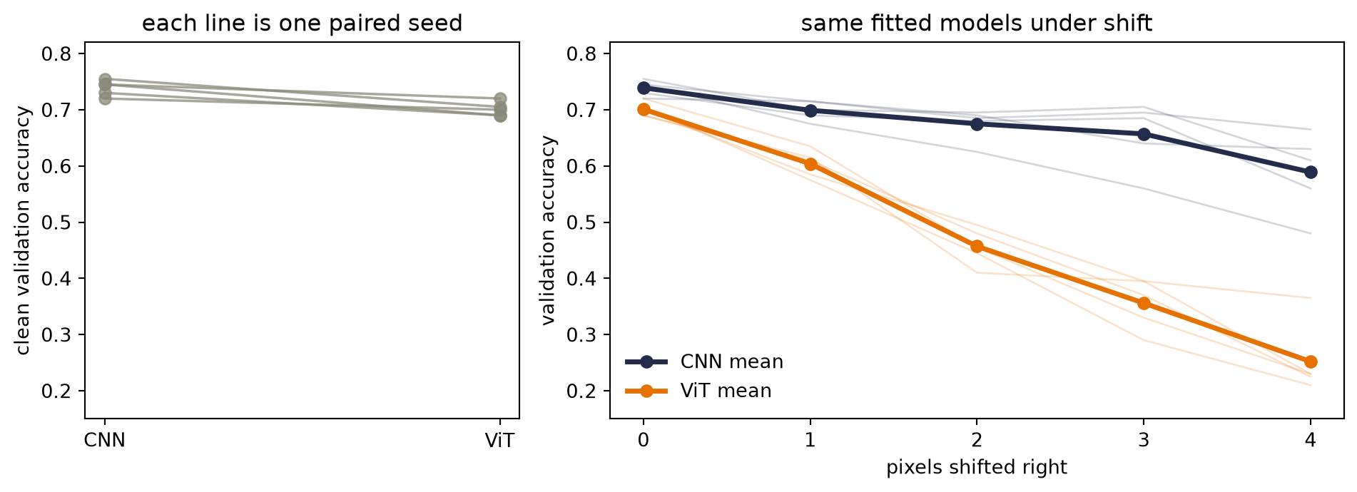
Figure 19.2: Five parameter- and schedule-matched runs on the fixed Chapter 6 split. Every line at left is one paired clean-validation comparison. At right, thin lines are individual seeds and thick lines are means under zero-padded right shifts; the operation also clips pixels at the right boundary. The CNN’s flatter curve is consistent with its local sharing and pooling, but the experiment does not isolate the causal effect of any one component.
Training and validation accuracy rank the two models in opposite orders. The ViT interpolates the fitting set in every run (100.0% mean training accuracy) but averages 70.1% on clean validation images. The CNN fits only 87.9% of the training labels under the shared recipe yet averages 73.9% on validation, winning all five paired comparisons. On the already-opened 600-image benchmark, the ViT averages 73.3% and the CNN 77.9%.
Under a four-pixel shift, the validation means separate much more: 25.2% for ViT and 58.9% for CNN. The zero-filled shift also pushes garment content off the right edge, so neither curve measures pure translation equivariance. Still, across the five fitted pairs the contrast is consistent with what Chapters 8–10 built into the CNN: local sharing, pooling, and a position-discarding global-average head.
WarningTrap: one regime, not a general ranking
These runs match the data split, parameter scale, optimizer, update count, minibatch order, and seeds. Their dot-product counts are close as well. They do not match architecture-specific tuning, every operation, or wall-clock cost. Neither model is pretrained, so this experiment does not test transfer from a pretrained checkpoint. The five runs vary initialization and order while holding one split fixed, so their spread does not estimate how results vary across different draws of the data. The 600-image benchmark was opened in earlier chapters and is descriptive, not a fresh final test. This experiment tells us what happened here; it does not rank CNNs and ViTs in general.
19.5 Scale changes the comparison
Now test the claim of Chapter 18 that pretraining is a regime, not an architecture. ViT keeps the encoder pattern but changes the tokens, source data, and task. In the original work, the decisive source task was supervised image classification, not BERT-style masked prediction, and the amount of source data changed the comparison.
The authors pretrained matched families on random subsets of JFT containing 9, 30, and 90 million images, plus the full 300-million-image dataset. These are four measured regimes, not points on a smooth curve we are free to invent. ViT-B/32 was slightly faster than the compared ResNet-50, performed much worse on the 9-million subset, and performed better at 90 million images and above. The analogous ViT-L/16 versus larger ResNet comparison followed the same regime change.
That does not prove “attention scales forever” or that data erases every useful prior. It demonstrates something narrower: the architecture ranking can reverse when the training regime changes. Our 1,000-example scratch run and the paper’s large-source-pretraining run answer different questions.
Three places a prior can re-enter
Pure global attention is not the only possible endpoint. Later designs put useful image structure back in at different places.
Where the prior enters
Example
What changes
Input
Hybrid CNN–ViT
A convolutional stem creates local feature tokens before global routing
Shifted local windows and a hierarchy constrain attention and control resolution cost
Training signal
DeiT
Strong augmentation and a convolutional teacher improve data efficiency without changing the student’s basic patch encoder
DeiT adds a teacher. The teacher provides another target, but it does not replace the ground-truth label, so a student can outgrow its teacher. In DeiT’s hard-distillation version, a distillation token learns from the teacher’s predicted class while [CLS] learns from the true class; the two heads are combined at inference. The teacher changes supervision, not the identity of the student.
ConvNeXt prevents a lazy conclusion in the opposite direction. Its study first modernized the training recipe, then progressively changed a ResNet toward design choices associated with contemporary Transformers. The training recipe alone raised the reported ResNet-50 ImageNet-1K accuracy from 76.1% to 78.8% before the architectural sequence was complete. Architecture, augmentation, optimization, and data interact: “CNN versus Transformer” is rarely a comparison between two isolated operators.
19.6 Scaling as design, scaling as forecast
Scaling names two different questions. EfficientNet asks how to enlarge one architecture family under a compute multiplier. Kaplan and Chinchilla ask how measured loss changes as parameters, data, and training compute grow. One is a design rule; the other is an empirical forecast.
Compound scaling: three knobs, one budget
Suppose a baseline convolutional network has depth \(d_0\), channel width \(w_0\), and input resolution \(r_0\). Scaling just one knob creates a bottleneck elsewhere: a deeper network still sees the same pixels, a wider network still has the same receptive-field schedule, and higher resolution asks an unchanged feature extractor to digest more detail. EfficientNet couples the knobs with one coefficient \(\phi\):
For ordinary dense convolutions, the leading operation count scales roughly as
\[
\operatorname{FLOPs}\propto d\,w^2r^2.
\]
Therefore one step in \(\phi\) multiplies the proxy by
\[
\alpha\beta^2\gamma^2\approx2.
\tag{19.4}\]
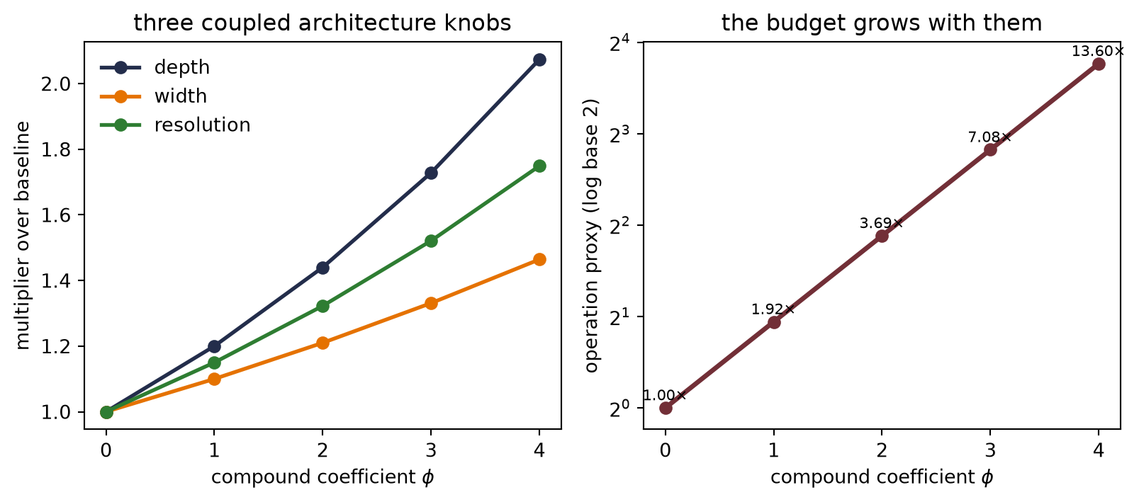
EfficientNet’s grid search on its baseline found approximately \(\alpha=1.2\), \(\beta=1.1\), and \(\gamma=1.15\), which give \(\alpha\beta^2\gamma^2=1.92027\): not exactly two, but close enough to serve as the intended budget step.
Set alpha, beta, and gamma and form the depth, width, resolution, and compute multipliers for phis 0 to 4.
Audit the EfficientNet compound-scaling constraint.
Figure 19.3: EfficientNet’s published compound multipliers. Each step in the compound coefficient \(\phi\) grows depth, width, and resolution modestly; their approximate convolutional-operation proxy grows by 1.92027 per step. These are normalized design multipliers, not measured accuracy or runtime.
The constants are an empirical design choice from a particular search and model family, not a law that every network must obey. When depth, width, and resolution all limit performance, increasing only one can waste compute.
19.7 A fitted power law, not a promise
Kaplan and colleagues asked a different question about decoder-only language models. When the other resources are not the bottleneck, how does test cross-entropy \(L\) change with non-embedding parameters \(N\), dataset tokens \(D\), or compute-optimally allocated training compute \(C_{\min}\)? Across their measured regime, the answer was well described by power laws:
Here \(N_c,D_c,C_c\) are fitted scale constants. Their values depend on the data, tokenizer, vocabulary, loss definition, and compute units; the small exponents are the more portable description of diminishing returns. These are conditional fits. The parameter curve assumes data is not the bottleneck, and the data curve assumes model capacity is not the bottleneck.
A power law becomes a straight line after taking logs:
\[
\log L=\log K-\alpha\log x.
\]
That makes extrapolation visually tempting: fit a line, extend it, and read a future loss. Extending the line still assumes that the conditions behind the fit hold.
Space 200 scales logarithmically from 1 to 1,000 and pair the parameter, token, and compute exponents with colors.
Turn the published Kaplan exponents into auditable multipliers.
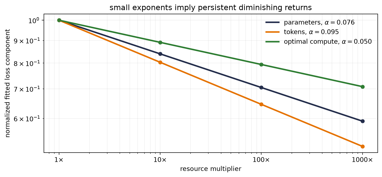
Figure 19.4: Implications of Kaplan et al.’s published exponents, normalized to one at the left endpoint. The markers and lines are calculated from the fitted laws, not raw training runs from this book. Even a thousand-fold resource increase leaves a substantial fraction of the fitted component, which is the arithmetic of diminishing returns.
Twice as many parameters multiplies the fitted parameter-limited loss by \(2^{-0.076}=0.949\), a 5.1% reduction. Doubling nonredundant data gives \(2^{-0.095}=0.936\), a 6.4% reduction. Doubling optimally allocated compute gives \(2^{-0.050}=0.966\), a 3.4% reduction. Comparing those percentages does not say that one parameter and one token have comparable cost or value; the units, constants, and constraints differ.
NoteA scaling law is a fitted conditional
The measured range, data distribution, objective, architecture family, optimizer, and the assumption that the other resources are not the bottleneck are part of the result. An extrapolation is a forecast that assumes those conditions still hold, not a guarantee. Kaplan’s basic one-variable fits above do not contain an explicit additive \(1.69\) floor; that constant belongs to the later Chinchilla joint fit.
Kaplan’s compute-optimal analysis suggested spending additional compute mostly on parameters:
That recommendation was influential, and it was later revised by a study designed to measure the allocation more directly.
19.8 Compute-optimal means balanced
Hoffmann and colleagues trained more than 400 language models while varying model size and token count. Their Chinchilla study estimated the compute-optimal frontier three ways.
Fitting approach
\(N_{\mathrm{opt}}\) exponent
\(D_{\mathrm{opt}}\) exponent
Minimum over training curves
0.50
0.50
IsoFLOP profiles
0.49
0.51
Parametric loss model
0.46
0.54
The exact answers differ, especially under long extrapolation, but all three move much more of the growing budget toward data than Kaplan’s \(0.73/0.27\) allocation. That agreement is the central result, not one ratio.
\(E\) is the fitted asymptotic loss floor for that distribution and objective; \(A/N^\alpha\) is the model-limited contribution; and \(B/D^\beta\) is the data-limited contribution. This decomposition is empirical. It is not a theorem that every language model has exactly three such terms.
For a dense Transformer, the study uses the approximation
\[
C\approx6ND,
\tag{19.6}\]
where \(C\) is training floating-point operations, \(N\) is non-embedding parameters, and \(D\) is processed training tokens. Recall from our derivation of backpropagation that a training step costs about three forward passes; with about two floating-point operations per parameter per token in each forward pass, that gives the factor six. It omits context-dependent and embedding details, so it is a planning equation rather than a profiler.
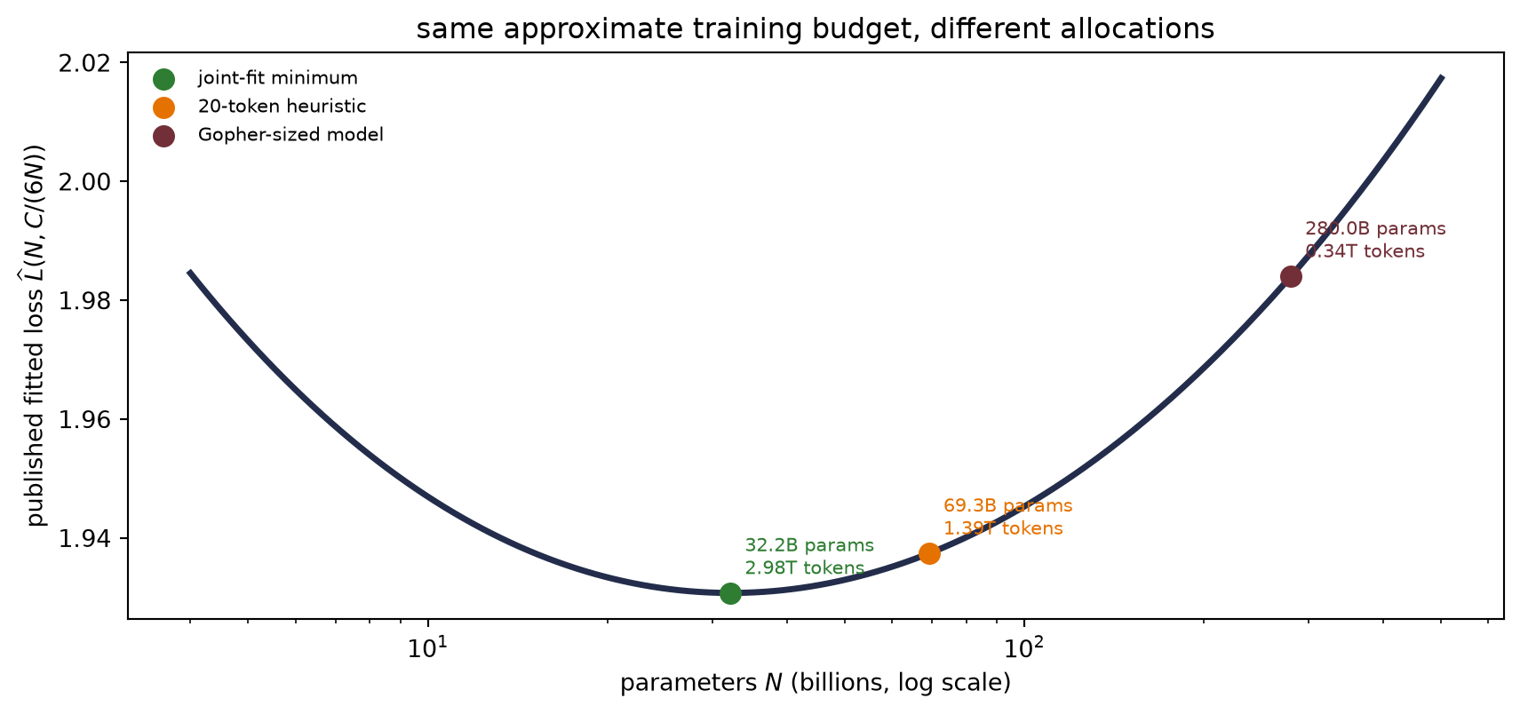
Fixing \(C\) forces \(D=C/(6N)\). Too large a model leaves too few tokens; too many tokens leave too little model. Substituting the constraint into Equation 19.5 and differentiating gives
The rounded constants imply exponents 0.452 and 0.548, close to the reported parametric-frontier fit of 0.46 and 0.54. At the reference budget \(C=5.76\times10^{23}\), this particular fitted surface reaches its minimum near 32.2 billion parameters and 2.98 trillion tokens. The other two methods put the optimal model size higher, roughly 40–70 billion parameters. The paper chose 70 billion parameters and 1.4 trillion tokens for Chinchilla, at the upper end of that range, partly for data and computational efficiency.
Set the published fit and budget, then compute the fitted optimum, the 20-token point, and the loss at 400 model sizes.
Define the reusable fitted_chinchilla_loss helper.
Report the joint-fit optimum beside the 20-token heuristic.
Figure 19.5: One reference iso-compute curve under the published Chinchilla parametric loss fit. The rounded joint fit reaches its mathematical minimum near 32.2B parameters; the separate 20-tokens-per-parameter heuristic lands near 69.3B/1.386T, close to the 70B/1.4T Chinchilla design. A Gopher-sized 280B allocation leaves far fewer tokens. The curve is a fitted surface evaluation, not a new training experiment.
The memorable 20 tokens per parameter comes from the near-balanced frontier estimated by the first two approaches: the paper’s table gives about 20.2 billion tokens for 1 billion parameters, 205.1 billion for 10 billion, and 1.5 trillion for 67 billion. If we impose the rounded heuristic \(D\approx20N\) at the \(5.76\times10^{23}\) budget, Equation 19.6 gives
That arithmetic is close to the actual Chinchilla design, but it is not the minimum of the rounded joint fit drawn above. Different fitting methods produced a broad range, and the authors made an engineering choice within it.
Gopher used about 280 billion parameters and 300 billion training tokens. Chinchilla used 70 billion parameters and 1.4 trillion tokens: four times fewer parameters and about 4.7 times more tokens, at approximately the same reported training budget. The smaller, longer-trained model achieved lower loss and outperformed the larger model across the paper’s broad evaluation suite. More parameters had not been the only way to spend the budget, and, in that regime, they had not been the best way.
WarningTwenty is not a constant of nature
The 20-to-1 ratio is an approximate rule from this study, model family, data, and frontier. The fitted methods do not agree exactly, and the ratio changes weakly with compute even inside the parametric model. Data quality, repetition, tokenization, objective, architecture, and downstream use can all move the useful allocation. Use the rule to challenge an obviously undertrained model, not to end the analysis.
19.9 Where the forecast stops
Scaling laws are powerful because they compress many expensive runs into a few fitted constants. That compression has limits.
Loss is not a capability map. A smoother aggregate cross-entropy curve does not tell us that every downstream skill appears smoothly, or exactly when a particular behavior becomes reliable.
Tokens are not interchangeable. A trillion repeated, low-quality, contaminated, or mismatched tokens need not buy what a trillion useful, diverse tokens buy. \(D\) counts processed tokens; it does not measure novelty or truth.
The law is local to a recipe and range. Change the architecture, optimizer, data mixture, context length, or evaluation distribution and the fitted constants can move. Extrapolation beyond the measured range adds uncertainty even when the line looks straight on log–log axes.
Training-optimal is not serving-optimal. Chinchilla allocates a training budget; it does not make the resulting backbone cheap to store, run, or adapt. That mismatch leads to Chapter 20: what can we change when moving every pretrained weight is no longer affordable?
This closes Part IV’s route from fixed lookup to global learned routing. We began with a memory bank in Chapter 14, learned how to score it, let every token query every other token, changed the visibility to pretrain representations, and finally let images enter as tokens. The operator was only half the story. The data and budget that train it are part of the model too.
NoteCheck yourself
Close the book for one minute and try each question below unaided.
For a 28×28 image with 4×4 patches, how many patch tokens appear before [CLS]?
Why does a matched toy CNN–ViT comparison describe a regime rather than declare a winner?
Under fixed training compute, why must parameter count and token count be chosen together?
19.10 Okay, so: patches become tokens, but regime still matters
An image can become a token sequence. Split it into \(P\times P\) patches, flatten to width \(CP^2\), and share a learned projection. Unfold-plus-linear is exactly a convolution with kernel and stride \(P\) after reshaping its weights.
ViT is an encoder transplant, not assumption-free learning. A learned [CLS] token that supplies a sequence-level representation, learned positions, pre-LayerNorm blocks, and a linear head reuse the Transformer pattern while retaining a small set of image and optimization biases.
Inductive bias is a trade. The five-seed Fashion comparison favors the CNN on clean validation and much more strongly under shift, but it covers one tiny scratch regime and ranks no architecture in general. Large supervised pretraining changed the comparison in the original ViT study.
An architecture’s brand name does not specify its training recipe. Hybrid stems, windowed routing, distillation, and ConvNeXt put priors in different places. Data, optimization, and operator design interact.
Scaling has two meanings here. EfficientNet’s compound rule coordinates depth, width, and resolution; empirical scaling laws forecast loss as parameters, tokens, and compute change. Both are resource-allocation tools, but they answer different questions.
Compute-optimal training balances model and data. Chinchilla revised the parameter-heavy Kaplan allocation, while also showing why a memorable 20-token heuristic must remain a heuristic. A fitted law carries its regime, assumptions, and uncertainty with it.
(Pencil.) A batch contains 12 RGB images at \(384\times384\). With \(P=16\) and model width \(d=768\), give the shapes of the raw batch, flattened patch tensor, projected patches, and sequence after [CLS]. Repeat the token and per-head score-entry counts for \(P=8\). By what factor did halving \(P\) change each count?
(Code.) Generalize the patch-equivalence cell to \(C=3\) and a rectangular image whose height and width are each divisible by \(P\). State the required unfold ordering, reshape a matrix \(\matr{E}\in\mathbb{R}^{CP^2\times d}\) into convolution weights, and assert equality to numerical tolerance. Explain why overlap appears when stride is smaller than \(P\).
(Audit.) Reproduce all five paired Fashion results and compute the paired clean-validation gaps, clean-to-four-pixel drops, and schedule hashes. Then change exactly one factor (add translated training examples) while keeping the split, seeds, initialization rule, model sizes, and minibatch schedules auditable. What question does the new comparison answer, and what still prevents a general CNN-versus-ViT claim?
(Pencil.) Using EfficientNet’s published constants, compute the depth, width, resolution, and operation-proxy multipliers at \(\phi=3\). Then use Kaplan’s exponents to compute the fitted component remaining after a 10-fold increase in parameters, data, and compute. Why can you not compare those three numbers as benefits per dollar?
(Pencil.) Starting from Equation 19.5 and Equation 19.6, derive Equation 19.7. Evaluate both the joint-fit optimum and the separate \(D=20N\) heuristic at a budget of \(1.2\times10^{22}\) FLOPs. Explain why disagreement between the answers is evidence to report rather than an algebra mistake, and name two deployment constraints neither calculation optimizes.
(Code.) Freeze one pinned Fashion CNN checkpoint from this chapter and fit one positive scalar temperature \(T\) on validation logits by minimizing NLL. With a fixed seed and fixed bin edges, draw validation and reused-benchmark reliability diagrams before and after scaling; report NLL, ECE, accuracy, and the fraction of class rankings that changed. The benchmark was opened in earlier chapters, so treat its results as exploratory. Verify numerically that dividing every class logit by the same positive \(T\) leaves argmax predictions unchanged. State what calibration improved and what it did not. This is post-hoc calibration of a frozen model, not Chapter 23’s training-time \(\gamma\). Named wrong answer: “better ECE means a more accurate classifier”; this post-hoc dial changes confidence, not the predicted class.
Appendix C supplies the missing count of bytes moved and the Roofline model, including why neither an operation count nor a dtype alone predicts elapsed time.↩︎