9  CNNs: Making the Filters Learnable

Chapter tools Lecture 4.1 · Convolutional Neural Networks·Lecture 4.2 · Coding Your First CNN·Download notebook·Open in Colab (opens in a new tab)

Chapter 8 applied a fixed local kernel with shared coefficients at every position. We now keep that spatial structure and optimize the coefficients against a task loss.

To do so, we declare the kernel coefficients to be learnable parameters. That single change is the core of this chapter. Everything else introduced here (channels, padding, stride and pooling) turns the learnable filter into a working network. By the end of the chapter we will have assembled LeNet, trained it on the Fashion-MNIST images of Chapter 6, and repeated that chapter’s shift experiment to test whether LeNet tolerates the shift better than the MLP did.

1. Load imports and the Fashion-MNIST subset.

import torch
import torch.nn as nn
import torch.nn.functional as F
import matplotlib.pyplot as plt
torch.set_num_threads(4)  # pinned: results depend on the CPU thread count

# [1]
torch.manual_seed(6050)
development = torch.load("../../data/fashion-train.pt")
holdout = torch.load("../../data/fashion-test.pt")
X_dev = development["X"].float().unsqueeze(1) / 255.0  # (1200, 1, 28, 28)
y_dev, classes = development["y"], development["classes"]
X_test = holdout["X"].float().unsqueeze(1) / 255.0     # (600, 1, 28, 28)
y_test = holdout["y"]

split = torch.randperm(len(X_dev), generator=torch.Generator().manual_seed(6050))
fit_idx, val_idx = split[:1000], split[1000:]
X_tr, y_tr = X_dev[fit_idx], y_dev[fit_idx]      # (1000,1,28,28), (1000,)
X_val, y_val = X_dev[val_idx], y_dev[val_idx]    # (200,1,28,28), (200,)

Note the shapes. In Part I our MLPs flattened every image into a vector of 784 pixels, discarding its two-dimensional arrangement at the first layer. A convolutional network keeps that geometry: the images stay rectangular grids, and they gain an explicit channel dimension, whose purpose we explain below.

WarningThe book’s batch convention: NCHW

Throughout this book, every image batch uses PyTorch’s NCHW order: (batch, channels, height, width). A single grayscale batch is therefore shaped (1, 1, 28, 28). Conv2d can also accept an unbatched (C, H, W) input, but keeping the batch dimension explicit makes downstream shapes predictable. The kernels of a conv layer are stored in a 4-D tensor too: (out-channels, in-channels, height, width). This bookkeeping is a common source of errors in convolutional code: when a shape error appears, count dimensions before changing anything else. Chapter 8’s conv2d helper hid this with x[None, None]; from here on we handle it in the open.

9.1 Learning a kernel from input–output pairs

Consider a game. A feature detector, one of the fixed filters of Chapter 8, is hidden from us; we observe only what it does: images go in, feature maps come out. Our job is to build a detector that matches it.

The tools of Part I suffice. A kernel applied by Equation 8.1 is just nine numbers entering a dot product \(\rightarrow\) the output is differentiable with respect to those numbers \(\rightarrow\) gradient descent applies. Start from a random kernel and run the loop we have run since Chapter 1: predict \(\rightarrow\) measure \(\rightarrow\) step.

1. Compute the hidden mystery kernel’s target maps on 256 garments and draw a small random K.
2. Recover a mystery kernel by gradient descent.

# [1]
mystery = torch.tensor([[-1., 0., 1.],
                        [-2., 0., 2.],
                        [-1., 0., 1.]])            # (don't peek)
imgs = X_tr[:256]                                  # (256, 1, 28, 28)
with torch.no_grad():
    target = F.conv2d(imgs, mystery[None, None])   # what the detector does

torch.manual_seed(0)
K = 0.1 * torch.randn(1, 1, 3, 3)
K_init = K.clone().squeeze()
K.requires_grad_(True)

lr = 0.5
# [2]
for step in range(601):
    pred = F.conv2d(imgs, K)                       # predict
    loss = F.mse_loss(pred, target)                # measure
    loss.backward()
    with torch.no_grad():                          # step
        K -= lr * K.grad
        K.grad.zero_()
    if step % 200 == 0:
        print(f"step {step:3d}   loss {loss.item():.2e}")

print(f"\nlearned kernel, rounded:\n{K.detach().squeeze().round(decimals=2)}")
print(f"max |learned - mystery| = {(K.detach().squeeze() - mystery).abs().max():.3f}")

step   0   loss 1.37e+00
step 200   loss 5.53e-04
step 400   loss 4.80e-05
step 600   loss 4.42e-06

learned kernel, rounded:
tensor([[-1.0100, -0.0000,  1.0100],
        [-1.9800, -0.0100,  1.9900],
        [-1.0100,  0.0100,  1.0000]])
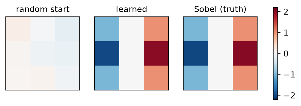
max |learned - mystery| = 0.018

The loss falls more than five orders of magnitude, and the learned kernel is the vertical Sobel detector to within 0.02 in every entry. Gradient descent, given nothing but input–output pairs, has recovered a filter that computer-vision researchers originally designed by hand.

Figure 9.1: The mystery-detector game. Left: the random starting kernel. Middle: the kernel gradient descent found from input–output pairs alone. Right: the hand-crafted vertical Sobel detector from Chapter 8. The middle kernel was fitted without any definition of an edge.

TipKernels learned from data

Deep learning for vision is that experiment at scale. Chapter 8 ended with the bottleneck: someone has to design the kernel, choosing its coefficients for a specific low-level operation such as smoothing or detecting intensity changes. What if the template were learnable? A convolutional network makes it learnable: it puts the coefficients on the gradient tape and fits them to the task loss, with machinery we have used since Chapter 4.

Two differences make the real thing harder than the game, not easier. First, the game was rigged: the target came from a known kernel, so a perfect answer existed and the loss surface was a clean convex bowl (the output is linear in the kernel \(K\), and squared error in a linear map is Chapter 1’s setting all over again). Second, and more important: in a real CNN, nobody supplies the target feature maps. The only supervision is the classification loss at the far end of the network. The gradient flows backward through every layer (exactly the mechanics of Chapter 5) and the kernels that emerge are whatever detectors the task loss favors. We chose Sobel here; a trained network may arrive at kernels that match no named filter.

Backpropagation through a convolutional layer applies the accumulation rule of Chapter 5: a quantity used in several places of a computation receives the sum of the gradients from all of them. The kernel is such a quantity. In the notation of Equation 8.1, write the kernel as \(V\) (the \(K\) of the game) and the output map as \(H\). The weight \([V]_{u,v}\) enters every output entry \([H]_{i,j}\), each time multiplied by the pixel \([X]_{i+u,\,j+v}\), so

\[ \frac{\partial L}{\partial [V]_{u,v}} \;=\; \sum_{i,j} \delta_{i,j}\,[X]_{i+u,\,j+v}, \qquad \delta_{i,j} = \frac{\partial L}{\partial [H]_{i,j}}, \]

with one more sum over the images of the batch. The gradient is itself a cross-correlation with the roles exchanged: the map of sensitivities \(\delta\) acts as the kernel and slides over \(X\), and its \(k \times k\) stops give the entries of \(\partial L/\partial V\). With the default reduction="mean" of F.mse_loss, each \(\delta_{i,j}\) carries a factor of one over the number of averaged entries. Weight sharing on the forward pass therefore means summed gradients on the backward pass: every patch of every image contributes to the update of the one shared template.

9.2 Channels: from one detector to many

One learnable kernel gives one feature map, and one feature map records one pattern: a vertical edge, a horizontal edge, a local average. The examples of fixed filters in Chapter 8 showed that an image carries many such patterns at once, and a classifier needs evidence about several of them at every position. A layer therefore applies several kernels to the same input, a team of specialized detectors, each producing its own feature map. Their responses at one position form a vector, and the representation gains a dimension: the channels.

Channels enter a convolutional layer at two places, with different roles:

• Out-channels add kernels. A conv layer with 6 output channels owns 6 independent kernels and produces a stack of 6 feature maps.
• In-channels let each kernel span the whole stack. The next layer’s input is that 6-deep stack, so the input at each position is a vector of 6 responses rather than one pixel. Each kernel of the next layer therefore grows a third dimension: a \(6 \times 5 \times 5\) volume that covers all six incoming maps at once.

For an input stack \(X\) with \(C_{\text{in}}\) channels, output feature map \(o \in \{1, \dots, C_{\text{out}}\}\) is

\[ [H_o]_{i,j} \;=\; b_o \;+\; \sum_{c=1}^{C_{\text{in}}}\; \Bigl(\,\sum_{u=-\Delta}^{\Delta}\;\sum_{v=-\Delta}^{\Delta} [V_{o,c}]_{u,v}\,[X_c]_{i+u,\,j+v}\Bigr), \tag{9.1}\]

and a pointwise activation follows; as in Chapter 8, the kernel is \(k \times k\) with \(k = 2\Delta + 1\). The inner double sum is the cross-correlation of Equation 8.1, applied to input channel \(c\) with the slice \(V_{o,c}\) of the kernel; the outer sum adds the \(C_{\text{in}}\) results, and \(b_o\) is the bias of output channel \(o\). The computation for one output pixel is one dot product between a \(C_{\text{in}} \times k \times k\) patch of the input and the \(C_{\text{in}} \times k \times k\) kernel of output channel \(o\), plus the bias \(b_o\). A dense layer of an MLP takes a dot product across all of its input features; a convolutional layer takes the same kind of dot product across all input channels but only a small spatial window, and slides it over the grid. The recipe of the layer (dot products, bias, activation) is the MLP’s; only the wiring of the linear part differs.

1. Build conv1 (1 to 6 channels) and conv2 (6 to 16), then feed one garment through both with ReLU.
2. Run one grayscale image through two conv layers.

# [1]
conv1 = nn.Conv2d(in_channels=1, out_channels=6, kernel_size=5, padding=2)
conv2 = nn.Conv2d(in_channels=6, out_channels=16, kernel_size=5)

x = X_tr[:1]                                   # (1, 1, 28, 28): one garment
h1 = F.relu(conv1(x))
h2 = F.relu(conv2(h1))
# [2]
print(f"input   {tuple(x.shape)}")
print(f"conv1   {tuple(h1.shape)}   kernels: {tuple(conv1.weight.shape)}")
print(f"conv2   {tuple(h2.shape)}  kernels: {tuple(conv2.weight.shape)}")

input   (1, 1, 28, 28)
conv1   (1, 6, 28, 28)   kernels: (6, 1, 5, 5)
conv2   (1, 16, 24, 24)  kernels: (16, 6, 5, 5)

Each kernel of conv2 spans all six maps of conv1, so it computes combinations of the first layer’s responses rather than of raw pixels. If earlier channels respond to edges of different orientations, a later channel can combine them into a response to corners or crossings. We build one such combination by hand on a filled square: two first-layer channels compute vertical and horizontal edge energy, and one second-layer kernel with equal positive weights on both channels sums them over a local window (Figure 9.2).

1. Make a filled-square image and compute edge magnitudes v and h with sobel_v and its transpose.
2. Run a corner detector built from two edge experts.

# [1]
square = torch.zeros(28, 28)
square[7:21, 7:21] = 1.0
sobel_v = torch.tensor([[-1., 0., 1.], [-2., 0., 2.], [-1., 0., 1.]])
v = F.conv2d(square[None, None], sobel_v[None, None], padding=1).abs()
h = F.conv2d(square[None, None], sobel_v.T.contiguous()[None, None], padding=1).abs()

# [2]
experts = torch.cat([v, h], dim=1)              # (1, 2, 28, 28): two reports
corner_k = torch.full((1, 2, 5, 5), 1 / 50)     # one kernel, spanning both
corners = F.conv2d(experts, corner_k, padding=2).squeeze()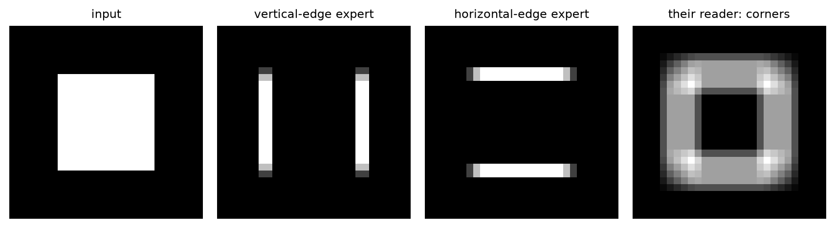

Figure 9.2: Combining two edge maps by hand. The input is a 28×28 image of zeros whose central 14×14 block (rows and columns 7 to 20) is set to 1. Two first-layer channels compute edge energy, the absolute response to the vertical Sobel kernel and to its transpose, each with padding 1. One second-layer kernel of shape 2×5×5, every entry 1/50 (Equation 9.1 with two input channels, padding 2), sums both edge maps over a local window, and its response is strongest near the square’s four corners.

For this square, the combined response is strongest near the corners, where both channels respond. The kernel only sums local edge responses, so a sufficiently strong response in either channel could also produce a large output. In a trained CNN, the coefficients of these combinations are learned from the task loss.

TipModules and functional operations

nn.Conv2d stores its kernels and biases as registered parameters. F.conv2d applies the operation using tensors supplied as arguments. Both support differentiation: the first experiment optimizes the kernel \(K\) directly, while LeNet uses modules to organize its trainable parameters.

9.3 Padding and stride: controlling the output size

Chapter 8 left a practical problem: a \(k \times k\) kernel on an \(n \times n\) image yields only \((n-k+1) \times (n-k+1)\) outputs, because the window must stay inside the frame. For one layer this is a small loss. For a deep stack it is fatal: unpadded \(5 \times 5\) convolutions take a \(28 \times 28\) image to 24, 20, 16, 12, 8 and then 4 pixels on a side, and a seventh layer would leave nothing.

Unpadded convolution also treats pixels unequally. A pixel enters one dot product for every window position that covers it, and near the border there are fewer such positions: a corner pixel is covered by a single window, an interior pixel by \(k^2\). Border pixels therefore contribute fewer terms to the output, and receive fewer gradient terms, than central ones.

The remedy is padding: a border of extra pixels, usually zeros, added around the input before the window slides. Padding serves two purposes. It decouples depth from shrinkage, so a network can be deep without its feature maps vanishing. It also narrows the border imbalance: for a \(3 \times 3\) kernel with one pixel of padding, a corner pixel enters 4 windows and an edge pixel 6, against 9 in the interior. For our \(5 \times 5\) kernels, a 2-pixel border keeps a \(28 \times 28\) image at \(28 \times 28\), which is why the first convolutional layer above uses padding=2.

Sometimes we want to shrink a map on purpose: coarser maps cost less computation, and every later window then covers more of the image. Stride moves the window \(s\) pixels at a time instead of one. A stride of 2 roughly halves each spatial dimension and divides the number of activations by about four. A strided convolution downsamples with learned weights; pooling downsamples with a fixed rule. Padding, kernel size and stride enter one formula:

\[ n_{\text{out}} \;=\; \left\lfloor \frac{n + 2p - k}{s} \right\rfloor + 1 . \tag{9.2}\]

Padding restores the output positions that the window would otherwise lose; stride skips stops on purpose. The numerator is the padded length minus the window, i.e. how far the window can travel; dividing by the step and flooring counts the stops; \(+1\) counts the starting position. Three worked cases make the arithmetic visible:

Watch the mechanism: counting the window's stops

A window 3 wide slides along a row of 8. With a border of one zero on each side and a stride of 2, how many stops does it make?

The code cell's three regimes, one row at a time: the formula works on each axis separately, so one dimension is the whole story.

\( n_{\text{out}} = \left\lfloor \frac{\class{os-travel}{n + 2p - k}}{\class{os-step}{s}} \right\rfloor \class{os-start}{+\,1} \)

Travel, divided by the step and floored, counts the hops; plus one counts where the window starts.

The calculation is readable without playback. Opening this panel loads the optional controls.

One row stands for one axis: a 2-D map runs the same count along its height and its width, which is why the code cell prints square shapes.

Scope and caveats

The row of 8, the window of 3 and the three (padding, stride) pairs are the shapes cell's; the counts 6, 8 and 4 are what that cell prints for the formula and for torch. The values inside the row do not matter to the count, so none are drawn.

The border is zeros, drawn dashed: padding adds positions for the window to stand on, not information. With stride 2 the last padded position is never a window start, and the floor is exactly that: a leftover shorter than one step buys no further stop.

Blue is the input, green the outputs, and the window and the ruler are neutral ink: nothing here is learned.

Check yourself. A 28-wide map meets a window of 3 with a border of 1 and stride 2. How many outputs along that axis?

14: the padded length is 30, the window can travel 27, so ⌊27 / 2⌋ + 1 = 13 + 1 = 14. The floor drops the last half step, and stride 2 halves the map, as a pooling layer would.

Transcript and keyboard help

1. A row of 8 inputs and a window 3 wide at its left end. Every stop of the window writes one output.
2. No padding, stride 1. The window can travel 8 minus 3, that is 5 cells, in hops of 1: 5 hops plus the starting position, 6 outputs.
3. Add one zero at each end. The padded row is 10 long, so the window can now travel 7.
4. Stride 1 again: 7 hops plus the start, 8 outputs, the input's own length.
5. Predict. Same border, stride 2: how many stops?
6. The window hops 2 at a time: 7 divided by 2 is 3 whole hops, plus the start, 4 outputs. The last padded cell is never a window start; the floor drops it.
7. The three regimes side by side: 6, 8 and 4, the counts the code cell prints.
8. Travel, divided by the step and floored, counts the hops; plus one counts where the window starts.

Silent; paused initially; 1.5× playback. Focus the animation pane: Space or K plays/pauses, arrows seek between beats, Home/End jump, Escape pauses. The scrubber and speed menu also work by keyboard. Reduced-motion mode holds each beat's finished state instead of moving between them.

1. Create a random 8×8 single-channel image x8 as a batch of one.
2. Implement the output-size formula, three regimes.

# [1]
x8 = torch.randn(1, 1, 8, 8)
# [2]
for p, s in [(0, 1), (1, 1), (1, 2)]:
    out = F.conv2d(x8, torch.randn(1, 1, 3, 3), padding=p, stride=s)
    n_out = (8 + 2 * p - 3) // s + 1
    print(f"n=8, k=3, p={p}, s={s}:  formula {n_out}  torch {tuple(out.shape[2:])}")

n=8, k=3, p=0, s=1:  formula 6  torch (6, 6)
n=8, k=3, p=1, s=1:  formula 8  torch (8, 8)
n=8, k=3, p=1, s=2:  formula 4  torch (4, 4)

9.4 Pooling: trading exact location for local tolerance

Chapter 8 established that stride-one convolution is translation-equivariant on the interior under matched boundary rules: shifting the input shifts the feature map. For classification, we also want the final decision to remain stable under the small, label-preserving shifts considered in Chapter 6.

Pooling summarizes a neighborhood of each feature map with one number. It reduces spatial resolution and can make some local rearrangements irrelevant to the pooled output. Whether that produces useful shift tolerance depends on the activations, window alignment, and subsequent layers. Two summaries are common, and neither has parameters:

• Max pooling keeps the largest activation in each window and discards the rest.
• Average pooling takes the mean of each window. The result is smoother, but a single large activation is diluted by small neighbors.

1. Fill a 4×4 grid t with the values 0 through 15, row by row.
2. Max and average pooling on a known grid.

# [1]
t = torch.arange(16.).reshape(1, 1, 4, 4)
# [2]
print(f"input:\n{t.squeeze()}")
print(f"max pool 2x2:\n{F.max_pool2d(t, 2).squeeze()}")
print(f"avg pool 2x2:\n{F.avg_pool2d(t, 2).squeeze()}")

input:
tensor([[ 0.,  1.,  2.,  3.],
        [ 4.,  5.,  6.,  7.],
        [ 8.,  9., 10., 11.],
        [12., 13., 14., 15.]])
max pool 2x2:
tensor([[ 5.,  7.],
        [13., 15.]])
avg pool 2x2:
tensor([[ 2.5000,  4.5000],
        [10.5000, 12.5000]])

The common configuration is the one above: \(2 \times 2\) windows with stride 2, non-overlapping, halving each spatial dimension. Our LeNet uses max pooling. Exercise 4 compares it with average pooling under the same training recipe.

How can this give local tolerance? Start with a deliberately clean construction in which max pooling removes the effect of a shift:

1. Place clues of 9 and 3 on a blank 4×4 scene, and build shifted with both moved one pixel right.
2. Run one constructed shift that pooling cannot see.

# [1]
scene = torch.zeros(1, 1, 4, 4)
scene[0, 0, 1, 0] = 9.0        # a strong clue, upper-left region
scene[0, 0, 2, 2] = 3.0        # a weaker clue, lower-right region

shifted = torch.zeros_like(scene)
shifted[0, 0, 1, 1] = 9.0      # both clues moved one pixel right
shifted[0, 0, 2, 3] = 3.0

# [2]
print(f"pooled original: {F.max_pool2d(scene,   2).squeeze().tolist()}")
print(f"pooled shifted:  {F.max_pool2d(shifted, 2).squeeze().tolist()}")

pooled original: [[9.0, 0.0], [0.0, 3.0]]
pooled shifted:  [[9.0, 0.0], [0.0, 3.0]]

Both activations moved, yet these particular pooled maps are identical: each isolated maximum stayed inside its \(2 \times 2\) window. That equality belongs to this construction, not to max pooling in general. A shift can change which values share a window, which maximum wins, or what crosses the boundary. Pooling can therefore absorb some jitter, but the amount depends on the activations and alignment; we test the complete network on shifted garments rather than assume tolerance.

WarningPooling reduces spatial detail

Pooling retains a coarse spatial grid while discarding information within each window. This can be useful when exact position is irrelevant to the task, but it can also remove distinctions needed for recognition or localization. The choice of pooling operation and resolution therefore belongs in the experimental comparison.

Watch the mechanism: the shift that pooling cannot see

Both activations move one pixel right — does the pooled map change? And one pixel down?

The 4 × 4 grid is this chapter's pool-invariance cell, printed above; blank cells are 0. The right shift is the chapter's shifted. The down shift is this panel's own computed case.

\( \displaystyle \featurepart{h_{i,j}} = \max_{(a,b)\,\in\,\class{pb-bin}{\mathcal{W}_{i,j}}} \featurepart{x_{a,b}} \)

Two pooled values changed: tolerance ends at the bin edge. Not invariance.

The calculation is readable without playback. Opening this panel loads the optional controls.

The equality is this construction's, as the chapter says: each isolated maximum stayed inside its 2 × 2 window. It is not translation invariance in general.

Scope and caveats

Only the two activations move, on the timeline rather than under a control; the bins, the window and the rule are fixed, and no kernel is learned, which is why nothing here is drawn in the colour reserved for a learnable parameter. The one-pixel move down is this panel's own computed case, made by applying the same 2 × 2 max-pool to the same two activations; the chapter does not print it. Under that move the 9 crosses from the upper-left bin into the lower-left one and the 3 does not, so exactly two of the four pooled values change. Tolerance is local and alignment-dependent, not invariance. How much tolerance pooling buys in a trained network is measured at the end of this chapter, not assumed here.

Check yourself. Move both activations one pixel up instead. What is the pooled map?

[9, 3, 0, 0]. The 9 stays inside its upper-left window, but the 3 crosses from the lower-right window into the upper-right one. The same rule as before: the pooled map is unchanged only until an activation crosses a bin boundary.

Transcript and keyboard help

1. Two activations on a 4 × 4 grid of zeros: 9 at row 1, column 0 and 3 at row 2, column 2. Every cell the picture leaves empty is 0. The grid is cut into four fixed 2 × 2 bins, drawn as heavy squares, and beside it stands the 2 × 2 pooled map with a question mark in each of its four cells. Each activation carries two dashed candidate moves, one right and one down. Before playing: after both activations move one pixel right, does the pooled map change?
2. Max-pool: each bin keeps only its largest value. One ray leaves the 9 and lands in the middle of its output cell's left edge; the four pooled values are written, that bin first: 9, 0, 0, 3.
3. The pooled map is recorded as a dashed copy under the live one, labelled before; both activations slide one pixel right and stay inside their bins; the four bins are pooled again.
4. Same pooled map, 9, 0, 0, 3, marked equal to the record: this shift is invisible to pooling.
5. The activations return home and the downward candidate move is drawn again. Before playing on: after both activations move one pixel down instead, does the pooled map survive?
6. The 9 crosses the edge from the upper-left bin into the lower-left one; the 3 stays in its bin. One ray leaves the 9's new cell into the lower-left output cell. Pooled again: 0, 0, 9, 3, marked not equal to the record, and the two bins that changed are ringed in wine on the live map and on the record together. The record's own label now reads before = after one pixel right, so both verdicts stand at once.
7. The two moves are drawn on the grid from the 9's home cell: the rightward one stays inside its bin, the downward one crosses into the next bin. Pooling buys local, alignment-dependent tolerance, not invariance.

Silent; paused initially; 1.5× playback. Focus the animation pane: Space or K plays/pauses, arrows seek between beats, Home/End jump, Escape pauses. The scrubber and speed menu also work by keyboard. Reduced-motion mode holds each beat’s state: the activations stand at exactly three positions — home, one pixel right, one pixel down — and never in between.

9.5 Receptive fields grow with depth

Stacking has one more consequence: it resolves the tension Chapter 6 left us with. Every kernel here is tiny and local: \(5 \times 5\). Yet recognizing a garment is a global judgment. Where does globality come from?

From depth. A neuron in the first feature map depends on a \(5 \times 5\) patch of the image: its receptive field. A neuron one layer up depends on a \(5 \times 5\) patch of feature maps, each pixel of which already summarizes a patch below \(\rightarrow\) its receptive field on the original image is wider. Pooling accelerates this: after a \(2\times2\)/stride-2 pool, neighboring pixels in the pooled map stand two original pixels apart, so every later window covers twice the ground. For our upcoming network the count runs: conv1 covers \(5 \times 5\) \(\rightarrow\) pooling nudges it to \(6 \times 6\) \(\rightarrow\) conv2’s \(5\times5\) window, at stride-2 spacing, expands it to \(14 \times 14\) \(\rightarrow\) the final pool reaches \(16 \times 16\), over half the frame in every direction, using only \(5 \times 5\) kernels.

Figure 9.3: Receptive fields by depth. Each box is the patch of the input that one unit depends on after a stage, drawn concentric for comparison. On the coat, the nested fields cross visible sleeves, torso, and boundary. One unit depends on a 5×5 patch after conv1, 6×6 after the first pool, 14×14 after conv2, and 16×16 after the final pool. Local wiring yields increasingly large fields; the dense head then combines all 25 overlapping final fields at once.

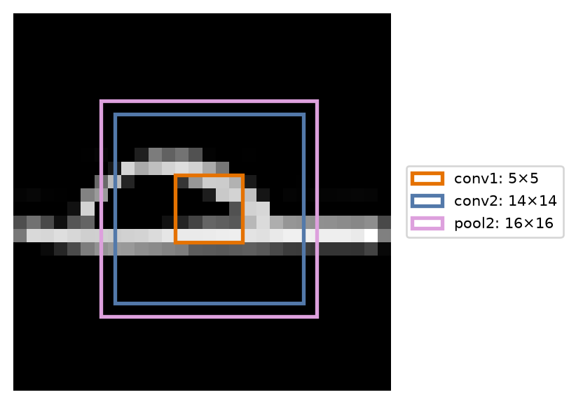
This is the compositional hierarchy of Chapter 3, now encouraged by the architecture. MLP layers also compose features. Convolution adds local connectivity and spatial sharing to that composition, and growing receptive fields let later layers compose earlier responses over larger regions. Learned channels often progress from edge-like patterns to textures and parts, but the architecture does not force those human labels. The CNN combines information across the frame gradually, through depth.¹

Watch the mechanism: channels say what, pooling says roughly where

Two edge detectors respond to the same square: one to vertical edges, one to horizontal edges. After max pooling shrinks their maps, can the network still tell the square's side from its top?

The two edge detectors from this chapter's corner detector, followed one step further: each edge map is max-pooled, as LeNet pools, before any later layer uses it.

\( \class{ww-channels}{[\predictionpart{H}_o]_{i,j}} = \Bigl|\sum_{u,v} [V_o]_{u,v}\,[\featurepart{X}]_{i+u,\,j+v}\Bigr|, \quad o \in \{\text{vertical}, \text{horizontal}\} \)\( \class{ww-pool}{[P_o]_{i,j} = \max_{(r,s)\,\in\,\text{block}(i,j)} [\predictionpart{H}_o]_{r,s}} \)

Channels say what was found; pooling says roughly where. Neither does the other’s job.

The calculation is readable without playback. Opening this panel loads the optional controls.

Nothing here is trained: the two edge detectors are the chapter's hand-built ones, and the pooling is the fixed 2 × 2 maximum LeNet uses.

Scope and caveats

The square, the vertical Sobel kernel and its transpose, and the two absolute-value edge maps are the chapter's corner-detector cell, which stacks them as two channels. That cell reads the stack at full resolution; this panel pools each edge map first, as LeNet does after every convolution, so the pooled values are computed here from the declared square and kernel and are not printed in the chapter.

Pooling takes one maximum per map and per 2 × 2 block. It shrinks the height and width by half, leaves the number of channels alone, and never compares one channel's number with another's. The counterfactual line, one maximum across both maps, is drawn only to show what that would cost: the square's side and its top would both read 4, and nothing downstream could tell them apart. What pooling does lose is position inside each block, which the chapter's pooling section and its replay measure separately.

Blue is the input image and green the two edge maps, pooled or not; the windows are neutral ink because nothing in them is learned here. In a trained network the edge detectors are learned kernels and there are six of them in LeNet's first layer, not two.

Check yourself. LeNet's first layer hands its pool six maps of 28 × 28. What shape leaves the pool, and how deep is each of the second layer's kernels?

6 × 14 × 14, and each second-layer kernel is 6 × 5 × 5. Pooling halves the height and width of every map and leaves all six channels in place; the next convolution is the step that combines the six maps, which is why its kernels are six deep.

Transcript and keyboard help

1. Predict. A white square on a black 28 by 28 image, and two empty maps: one for a vertical-edge detector, one for a horizontal-edge detector. After pooling, will the network still be able to tell the square's side from its top?
2. Two detectors, one window. A three by three window sweeps the image once, and at every position both detectors write a reading into their own map. The vertical map lights the square's left and right sides; the horizontal map lights its top and bottom.
3. One spot, two readings. At a point on the square's left side the pair reads 4 and 0; on its top, 0 and 4; at its corner, 3 and 3. The stack's depth says which edges are present at a spot.
4. Pool each map. A two by two window runs through both maps in step, and each map keeps the largest of its own four numbers. Both maps shrink from 28 by 28 to 14 by 14; there are still two of them.
5. Hold. The probe sits on the pooled block at the square's side and on the pooled block at its top. Predict: can the pooled pair still tell them apart?
6. Yes. The side block reads 4 and 0 and the top block 0 and 4, because each map was pooled on its own. Had one maximum been taken across both maps, both blocks would read 4 and the difference would be gone.
7. The shapes. The convolution took one channel of 28 by 28 to two channels of 28 by 28; pooling took two channels of 28 by 28 to two channels of 14 by 14. Convolution changed the depth, pooling the space.
8. Channels say what was found; pooling says roughly where. The next convolution is the step that reads the channels together.

Silent; paused initially; 1.5× playback. Focus the animation pane: Space or K plays/pauses, arrows seek between beats, Home/End jump, Escape pauses. The scrubber and speed menu also work by keyboard. Reduced-motion mode holds each beat's finished state instead of moving between them.

9.6 LeNet: the whole machine

The canonical blueprint is LeNet, Yann LeCun’s digit-reading network, and its rhythm is the CNN design pattern to this day: convolve, shrink, deepen; repeat; then decide. Spatial size falls (28 \(\rightarrow\) 14 \(\rightarrow\) 5) while feature depth grows (1 \(\rightarrow\) 6 \(\rightarrow\) 16): the network trades “where” for “what” stage by stage, until a small dense head maps the final \(16 \times 5 \times 5\) summary to class scores.

Watch the mechanism: LeNet's tensor, one layer at a time

The text says the maps shrink 28 → 14 → 5. The second convolution has no padding: what size does it hand to the second pool?

One garment's tensor through the code below, layer by layer: each convolution sets the depth, each pool and each unpadded window sets the size.

\( \class{lf-size}{n_{\text{out}} = \left\lfloor \frac{n + 2p - k}{s} \right\rfloor + 1} \)\( \class{lf-kernels}{\text{depth}_{\text{out}} = \text{number of } \parameterpart{\text{kernels}}} \)

Convolve, shrink, deepen; repeat; then decide.

The calculation is readable without playback. Opening this panel loads the optional controls.

These are shapes, not values: the boxes show how big each tensor is, and nothing here is trained or evaluated.

Scope and caveats

Every shape comes from the lenet cell's layers and matches its shape comments: the output-size formula gives the height and width, and the number of kernels gives the depth. The chapter's prose rounds the size path to 28, 14, 5; the unpadded second convolution's 10 × 10 sits between 14 and 5.

A box's face is drawn in proportion to height and width and its depth to the number of channels; the head's bars are in proportion to their length. ReLU follows each convolution and the first two dense layers without changing any shape, so it is named on the arrows and not drawn.

Blue is the input, green each computed tensor, and orange the learned weights' counts and shapes; the arrows are neutral ink.

Check yourself. fc1 reads the flattened summary and has 120 outputs. How many parameters does it hold?

48,120: a 120 × 400 weight matrix, one weight for each of the 400 flattened numbers and each output, plus 120 biases. That is more than eighteen times the 2,572 parameters of both convolutions together, which is the imbalance the parameter audit below prints.

Transcript and keyboard help

1. A one-channel 28 by 28 image goes in; ten votes come out. The shape is followed through every layer.
2. conv1: six 5 by 5 kernels with padding 2. Height and width stay 28, since 28 plus 4 minus 5, plus 1, is 28. Six kernels make six maps: 6 by 28 by 28.
3. Max pooling with a 2 by 2 window and stride 2 halves each map: 6 by 14 by 14.
4. Predict. conv2 has sixteen 5 by 5 kernels, each 6 deep, and no padding. What size comes out of 14 by 14?
5. 10 by 10: 14 minus 5, plus 1. Sixteen kernels make sixteen maps: 16 by 10 by 10.
6. Pooling again gives 16 by 5 by 5. The size fell from 28 to 5 while the depth grew from 1 to 16.
7. Flatten the 16 by 5 by 5 summary into 400 numbers. Three dense layers take it to 120, 84 and finally 10 logits, one per class.
8. Convolve, shrink, deepen; repeat; then decide.

Silent; paused initially; 1.5× playback. Focus the animation pane: Space or K plays/pauses, arrows seek between beats, Home/End jump, Escape pauses. The scrubber and speed menu also work by keyboard. Reduced-motion mode holds each beat's finished state instead of moving between them.

1. LeNet.

# [1]
class LeNet(nn.Module):
    def __init__(self):
        super().__init__()
        self.conv1 = nn.Conv2d(1, 6, 5, padding=2)  # (N,1,28,28)->(N,6,28,28)
        self.conv2 = nn.Conv2d(6, 16, 5)            # (N,6,14,14)->(N,16,10,10)
        self.fc1 = nn.Linear(16 * 5 * 5, 120)
        self.fc2 = nn.Linear(120, 84)
        self.fc3 = nn.Linear(84, 10)

    def forward(self, x: torch.Tensor) -> torch.Tensor:
        x = F.max_pool2d(F.relu(self.conv1(x)), 2)   # -> (N, 6, 14, 14)
        x = F.max_pool2d(F.relu(self.conv2(x)), 2)   # -> (N, 16, 5, 5)
        x = x.flatten(1)                             # -> (N, 400)
        x = F.relu(self.fc1(x))
        x = F.relu(self.fc2(x))
        return self.fc3(x)                           # logits, (N, 10)

Every line is a tool we already own: Equation 9.1 twice, Equation 9.2 behind the choice of padding=2, pooling twice, then Chapter 3’s MLP as the decision head. The convolutional layers form the backbone, and fc1 through fc3 replace Chapter 2’s single linear head with a small MLP. Per Chapter 2’s advice, the model returns raw logits and lets F.cross_entropy handle the probabilities.

NoteLeNet, then and now

The LeNet family (LeCun and colleagues, 1989–1998) began by reading handwritten ZIP codes for the US Postal Service, and its mature form, LeNet-5, went on to read a substantial share of America’s bank checks. Our variant keeps the classic skeleton but changes its internals: ReLU where the original used sigmoid-family activations (Chapter 3, Chapter 5), max pooling where it used subsampling based on averaging, Adam as the optimizer. Our later CNNs add one more modern stabilizer, batch normalization, which we meet properly in Chapter 10.

Before training, we count the parameters: weight sharing in Chapter 8 should save many, and Chapter 6’s MLP is the yardstick:

1. Define the reusable make_mlp helper.
2. Instantiate a fresh LeNet and a fresh MLP from make_mlp.
3. Parameter audit, LeNet vs. Chapter 6’s MLP.

# [1]
def make_mlp() -> nn.Sequential:
    return nn.Sequential(nn.Flatten(),
                         nn.Linear(784, 256), nn.ReLU(), nn.Linear(256, 10))

# [2]
lenet, mlp = LeNet(), make_mlp()
# [3]
for name, p in lenet.named_parameters():
    print(f"{name:14s} {str(tuple(p.shape)):16s} {p.numel():>7,}")
n_conv = sum(p.numel() for n, p in lenet.named_parameters() if "conv" in n)
n_lenet = sum(p.numel() for p in lenet.parameters())
n_mlp = sum(p.numel() for p in mlp.parameters())
print(f"\nLeNet: {n_lenet:,} parameters ({n_conv:,} of them convolutional)")
print(f"MLP:   {n_mlp:,} parameters")

conv1.weight   (6, 1, 5, 5)         150
conv1.bias     (6,)                   6
conv2.weight   (16, 6, 5, 5)      2,400
conv2.bias     (16,)                 16
fc1.weight     (120, 400)        48,000
fc1.bias       (120,)               120
fc2.weight     (84, 120)         10,080
fc2.bias       (84,)                 84
fc3.weight     (10, 84)             840
fc3.bias       (10,)                 10

LeNet: 61,706 parameters (2,572 of them convolutional)
MLP:   203,530 parameters

These parameter counts can be read two ways. Against the MLP of Chapter 6, rebuilt here as make_mlp (the network of that chapter with an nn.Flatten() in front: 784 inputs, 256 hidden ReLU units and 10 outputs), LeNet carries 61,706 parameters to the MLP’s 203,530 (less than a third) while performing far richer spatial computation. This is the saving that Chapter 8’s matrix view showed. Within LeNet, the two convolutional layers, which compute the spatial features, hold 2,572 parameters (about 4%), and the dense head holds the rest. We reduce that imbalance in Chapter 10, where modern architectures go deeper in convolution and lighter in the head.

Now train both models under one shared optimization recipe: same fitting split, optimizer, minibatch size, number of epochs, and therefore number of parameter updates. The comparison does not match parameter count or floating-point work; a convolution and a dense layer spend different computation per update. Architecture is the intended difference; compute is not controlled:

1. Define the reusable helpers: train_model and accuracy.
2. Run one recipe, two architectures.
3. Print train and validation accuracy for the MLP and for LeNet.

from dlbook.supervised import fit_supervised   # Listing 4.1

# [1]
def train_model(
    model_fn, X_fit: torch.Tensor = X_tr, y_fit: torch.Tensor = y_tr,
    epochs: int = 150, batch: int = 128, seed: int = 6050
) -> nn.Module:
    # Listing 4.1 verbatim; this chapter's deltas are the budget (150
    # epochs, batch 128) and, below, the models that get trained.
    return fit_supervised(
        model_fn, X_fit, y_fit, epochs=epochs, batch=batch, seed=seed
    )

@torch.no_grad()
def accuracy(model: nn.Module, X: torch.Tensor, y: torch.Tensor) -> float:
    model.eval()
    return (model(X).argmax(1) == y).float().mean().item()

# [2]
mlp = train_model(make_mlp)
lenet = train_model(LeNet)
# [3]
for name, model in [("MLP  ", mlp), ("LeNet", lenet)]:
    print(f"{name}  train {accuracy(model, X_tr, y_tr):.1%}   "
          f"validation {accuracy(model, X_val, y_val):.1%}")

MLP    train 100.0%   validation 75.5%
LeNet  train 99.5%   validation 74.5%

Read the clean-validation column: the MLP scores 75.5% and LeNet 74.5% in this single seeded run. A one-point difference is descriptive, not an uncertainty estimate, so it does not establish which architecture has higher expected clean accuracy. Both models nearly interpolate the fitting split. Our small-data regime makes a narrower point: LeNet reaches comparable clean accuracy with less than a third of the parameters. The shift experiment now compares the two models on shifted garments.

9.7 LeNet under the two-pixel shift

In Chapter 6, shifting every validation image two pixels to the right took our MLP from 76.0% to 46.5% accuracy. We now give LeNet the same test. Retrained here on LeNet’s schedule, the MLP starts from 75.5% clean validation accuracy and LeNet from 74.5%, so the two begin level. The question is whether the convolutional structure makes the classifier more tolerant of the shift.

1. Define the reusable shift_right helper.
2. Compute acc_mlp and acc_cnn, validation accuracy under right shifts of 0 to 4 pixels.
3. Plot accuracy vs. shift, both models.

# [1]
def shift_right(X: torch.Tensor, px: int) -> torch.Tensor:
    out = torch.zeros_like(X)
    if px == 0:
        return X.clone()
    out[..., px:] = X[..., :-px]
    return out

# [2]
shifts = list(range(5))
acc_mlp = [accuracy(mlp, shift_right(X_val, s), y_val) for s in shifts]
acc_cnn = [accuracy(lenet, shift_right(X_val, s), y_val) for s in shifts]
# [3]
for s in shifts:
    print(f"shift {s}px:   MLP {acc_mlp[s]:.1%}   LeNet {acc_cnn[s]:.1%}")

plt.figure(figsize=(5.5, 3.2))
plt.plot(shifts, acc_mlp, "o-", color="#E57200", lw=2, ms=7, label="MLP (Ch. 6)")
plt.plot(shifts, acc_cnn, "s-", color="#232D4B", lw=2, ms=7, label="LeNet")
plt.axhline(0.1, ls=":", color="#B8B8A8")
plt.xlabel("shift (pixels right)"); plt.ylabel("validation accuracy")
plt.ylim(0, 0.9); plt.xticks(shifts); plt.legend()
plt.tight_layout(); plt.show()

shift 0px:   MLP 75.5%   LeNet 74.5%
shift 1px:   MLP 64.0%   LeNet 66.0%
shift 2px:   MLP 42.0%   LeNet 57.5%
shift 3px:   MLP 27.0%   LeNet 42.0%
shift 4px:   MLP 18.5%   LeNet 23.0%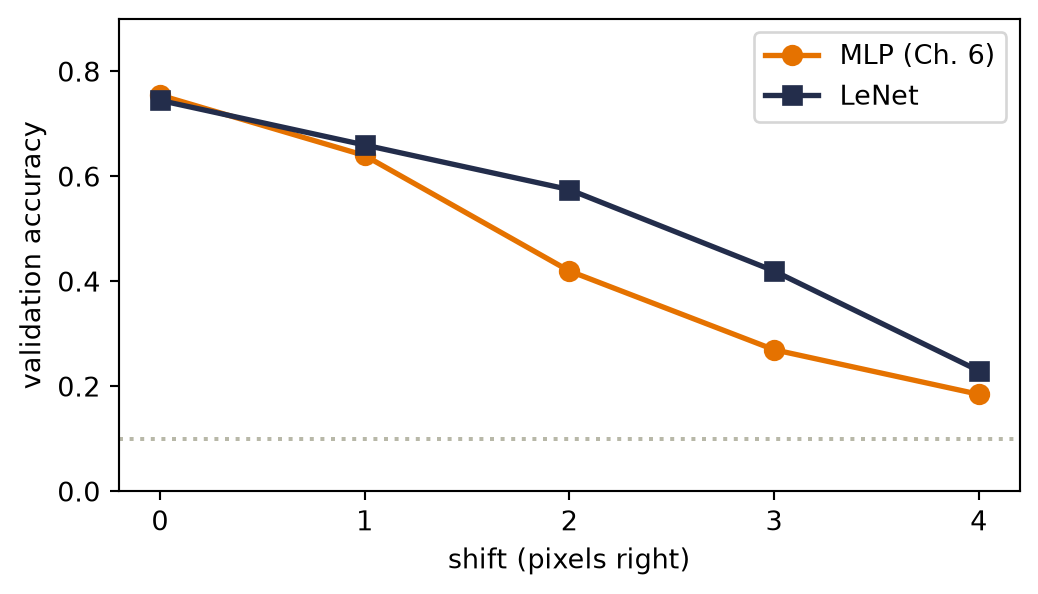

Figure 9.4: Validation accuracy under right shifts. Both architectures use the same optimizer schedule, though not matched compute. At two pixels the MLP falls from 75.5% to 42.0%, while LeNet falls from 74.5% to 57.5%. The dotted line is chance.

LeNet stays above the MLP at every nonzero shift, and the gap is largest at two and three pixels. At one pixel the two are close, 66.0% for LeNet and 64.0% for the MLP. At two pixels the MLP loses 33.5 points and LeNet 17.0; at three, LeNet scores 42.0% against 27.0%, and at four, 23.0% against 18.5%. These numbers come from one deterministic validation split, not a sampling distribution, but the within-run contrast is large.

The comparison changes the complete architecture, so it does not isolate the contributions of locality, weight sharing, pooling or the classifier head. Several operations can still introduce shift sensitivity: cropping and padding affect the responses at the border, pooling depends on window alignment, and the dense head gives each spatial position retained after flattening its own weights. Chapter 10 replaces that position-sensitive head with global pooling.

In Chapter 6, the MLP’s first-layer weights were full-frame templates with broad, diffuse patterns. Figure 9.5 shows the six \(5 \times 5\) kernels of LeNet’s first layer and, under each, its feature map after the ReLU on the coat of Figure 9.3, a validation image.

1. Extract first-layer kernels and their feature maps.

# [1]
example_index = 3                                   # the Figure 9.3 coat
img = X_val[example_index:example_index + 1]
with torch.no_grad():
    fmaps = F.relu(lenet.conv1(img)).squeeze(0)     # (6, 28, 28)
kernels = lenet.conv1.weight.detach().squeeze(1)    # (6, 5, 5)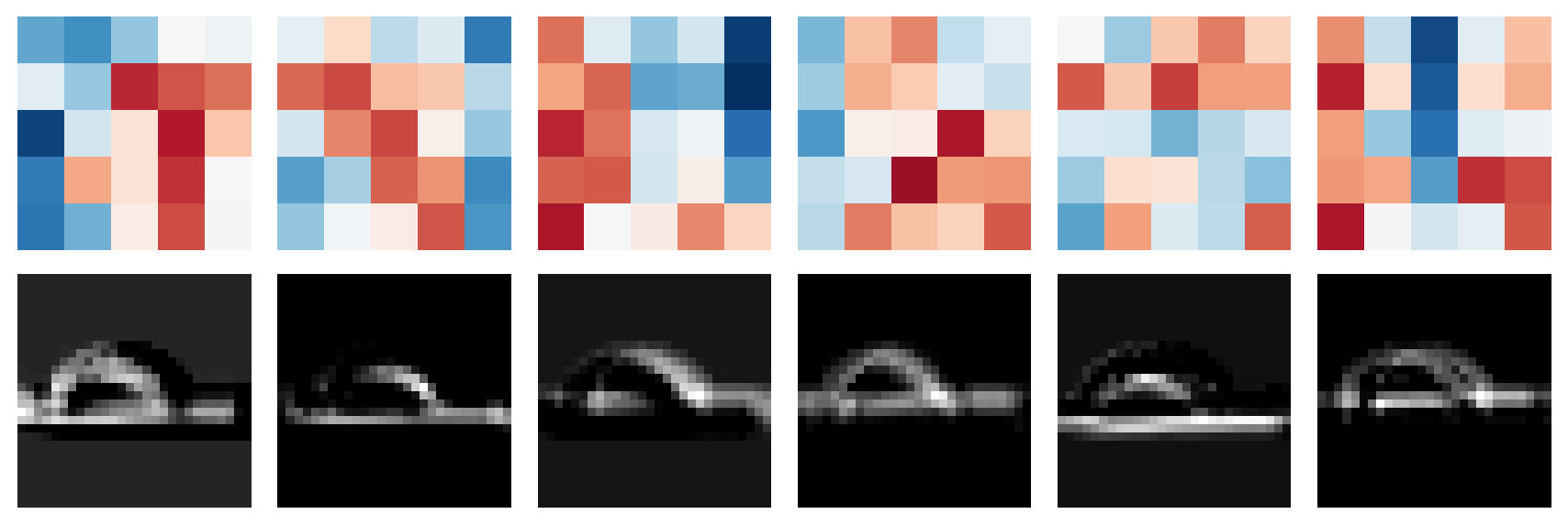

Figure 9.5: What LeNet’s first layer learned. Top: six first-layer 5×5 kernels (red positive, blue negative). Bottom: their feature maps on the coat of Figure 9.3, a validation image whose sleeves and torso make spatial responses easy to compare. The maps respond differently, but several kernels remain diffuse and should not be over-interpreted.

The six local kernels produce distinct response maps on the same image. Some show directional structure; others remain noisy enough that naming them as detectors would claim more than this one run supports. Nobody designed them: they result from optimizer steps on the classification loss, with gradients flowing backward through Equation 9.1.

9.8 One sealed test check

With both architectures, the optimizer schedule, the shift size and the two reported metrics fixed, we refit each model on all 1,200 development images with the same training budget, open the 600-image test set once, and score each refit model on the clean test images and on the same images shifted two pixels right. Sealed is chapter-local here: these 600 images also serve other chapters as an endpoint, as the experiment interlude explains, but no choice in this chapter looked at them.

1. Run one final test-set check.
2. Print clean and two-pixel-shifted test accuracy for the refit MLP and LeNet.

# [1]
mlp_final = train_model(make_mlp, X_dev, y_dev)
lenet_final = train_model(LeNet, X_dev, y_dev)
# [2]
for name, model in [("MLP  ", mlp_final), ("LeNet", lenet_final)]:
    print(f"{name}  clean {accuracy(model, X_test, y_test):.1%}   "
          f"shift-2 {accuracy(model, shift_right(X_test, 2), y_test):.1%}")

MLP    clean 82.2%   shift-2 41.8%
LeNet  clean 82.5%   shift-2 62.3%

The sealed check confirms the validation comparison. On clean test images the MLP scores 82.2% and LeNet 82.5%, a descriptive 0.3-point gap from one seed. Under the predeclared two-pixel shift the MLP falls to 41.8% and LeNet to 62.3%, with less than a third of the MLP’s parameters.

NoteCheck yourself

Close the book for one minute and rebuild the CNN.

• Which kernel entries become learnable, and which convolutional structure remains built in?
• What do channels, pooling, and receptive-field growth each contribute?
• What does the shift comparison establish under this recipe, and why does it not isolate one architectural constraint?

9.9 Okay, so: the kernel became learnable

1. One change: the kernel’s numbers became parameters. Gradient descent can recover a hand-crafted detector from data (our rigged game) and, more importantly, learn kernels nobody designed, supervised only by the task loss at the far end.
2. Channels turn one detector into many: out-channels stack the feature maps of several kernels; in-channels let each next-layer kernel combine all maps at once (Equation 9.1).
3. Padding and stride are the shape budget: \(n_{\text{out}} = \lfloor (n + 2p - k)/s \rfloor + 1\) (Equation 9.2). Padding lets networks go deep without shrinking to nothing; stride shrinks on purpose.
4. Pooling summarizes each window by one number: max pooling keeps the largest activation and discards its exact position within the window. Any resulting shift tolerance depends on the activations, window alignment, and later layers.
5. Receptive fields grow with depth: \(5 \rightarrow 6 \rightarrow 14 \rightarrow 16\) in our LeNet. Stacked local layers cover more of the frame at each stage. Like the MLP layers of Chapter 3, they compose features, now with local connectivity and spatial sharing.
6. The verdict: on the sealed test set, one seed puts clean accuracy at 82.2% for the MLP and 82.5% for LeNet; this does not establish an expected clean-accuracy difference. Under the predeclared two-pixel shift, the same models score 41.8% and 62.3%. Under this training recipe, LeNet achieves higher accuracy on the shifted images with fewer parameters. This compares the two complete models, rather than isolating one architectural constraint.

Most of LeNet’s parameters remain in its dense head, and its accuracy still declines under image shifts. The next chapter examines smaller classifier heads, deeper convolutional networks, and the training choices needed to compare them.

Sources and further reading

• LeCun et al., “Gradient-Based Learning Applied to Document Recognition” (1998): the primary LeNet account, including the architecture’s document-recognition setting.
• Fukushima, “Neocognitron: A Self-organizing Neural Network Model” (1980): historical context for alternating feature extraction and spatial tolerance.
• Zeiler and Fergus, “Visualizing and Understanding Convolutional Networks” (2014): methods and evidence for inspecting learned convolutional features without over-reading a single filter image.
• Dumoulin and Visin, “A Guide to Convolution Arithmetic for Deep Learning” (2016): a compact companion for checking convolution, pooling, and receptive-field shapes.

Exercises

1. (Pencil.) Run Equation 9.2 through LeNet layer by layer, starting from \(28 \times 28\): verify every shape comment in the LeNet class, then verify the parameter counts of conv1 and conv2 from the table (weights and biases).
2. (Pencil.) Verify the receptive-field growth \(5 \rightarrow 6 \rightarrow 14 \rightarrow 16\). (Track two numbers per stage: the field size, and the jump, the spacing in input pixels between neighboring units, which each stride-2 pool doubles.) Then show that no convolutional or pooling unit in LeNet has a receptive field covering the full \(28 \times 28\) frame. Where does globality finally enter the network?
3. (Code.) Play the mystery-detector game with the \(3 \times 3\) blur kernel as the target. Does gradient descent recover it as cleanly as Sobel? Now rerun with only 8 training images instead of 256. What happens to the recovered kernel, and what does that say about data volume versus parameter identifiability?
4. (Code.) Swap LeNet’s max pooling for average pooling and retrain. Compare clean accuracy and the shift curve. Which changes more, and does the result match the contrast drawn above between keeping the largest activation and averaging the window?
5. (Pencil.) The final dense head receives 25 spatial positions per feature map. Explain why this can reintroduce shift sensitivity after equivariant convolutions. Describe what information a position-insensitive head would keep and discard; we will build one in Chapter 10.

---

1. Attention (Chapter 15) combines information across the whole input in a single step, at a different cost.