The autoencoders of Chapter 11 encode an input of one fixed size in a single pass. When a sequence grows by one element, they have no operation that updates the code already computed. In this chapter we learn such an operation: a rule that combines a fixed-width summary of the elements seen so far with the next element to give the new summary.
Text, audio, and sensor measurements are sequences: ordered lists of elements whose length varies from one example to the next. When the elements are symbols from a fixed set, such as the characters or words of a text, each element is called a token. For the streaming models developed in this chapter, we use six design goals to compare possible architectures:
Any length. Accept a sequence of unknown length, with no maximum length imposed by the architecture. Memory and compute still bound what can be processed.
Order. Allow the representation to distinguish the same elements in different orders. The sentences “the dog bit the man” and “the man bit the dog” contain the same words but report different events, so a representation that ignores word order cannot separate them.
Streaming. Update as each element arrives, so that an output for the elements seen so far is always available.
Parameters independent of length. The rule that reads position 17 should be the rule that reads position 18, so a longer sequence costs no new parameters.
Reach. Let the output at the current step depend on inputs arbitrarily far back, not only on the most recent ones. In other words, the architecture sets no limit on the model’s context length, the number of past steps whose inputs enter the computation of the current output. That an early input enters the computation does not by itself ensure that its information is retained or that the dependency can be learned.
Trainable reach. Make such a dependency learnable. If the correct output at the current step depends on an input many steps back, the gradient of the loss must keep a usable size as backpropagation carries it back across those steps to the early input: if it shrinks to nearly zero, the parameter updates carry almost no information about the dependency, and the reach exists only on paper.
The interlude’s one-shot autoencoder fails the first and third outright: it needs a maximum length, and it cannot finish before the last element arrives. Recurrence asks us to make the carried summary learnable: rather than compressing once, the model learns how to revise its memory after each new element.
Four earlier tools do most of the work in this chapter: the kernel shared across space in Chapter 8 and Chapter 9, which becomes one rule shared across time; the product of Jacobians that vanished down deep networks in Chapter 5, now measured across time; the softmax and the sigmoid of Chapter 2, which become a distribution over the next character and multiplicative factors that control what a recurrent state keeps; and the additive form of the residual connection of Chapter 10, which a recurrent architecture applies along the sequence.
12.1 Stretching the old toolkit
A window. We predict the next element \(\vect{x}_{t+1}\) from the last \(k\), \(\vect{x}_{t-k+1}, \dots, \vect{x}_t\), by sliding a width-\(k\) window along the sequence and feeding each snapshot to an MLP. This is autoregression, and the sliding is a one-dimensional convolution: locality, transplanted from space to time. Windows are useful (they power real forecasting systems), but they inherit locality’s blind spot: anything older than the last \(k\) elements lies outside the window and cannot affect the prediction. The window’s context length is therefore \(k\), and no fixed \(k\) covers every dependency, as in the sentence “The company whose first-day price we recorded back in January finally …”. In the list’s terms, the window meets the first four goals and fails the fifth, and buying more reach costs parameters.
A function per timestep. Next we let the model change over time: we learn \(f_1\) for step one, \(f_2\) for step two, and so on, and each passes a summary forward, \(\vect{h}_t = f_t(\vect{h}_{t-1}, \vect{x}_t)\). The parameter count now grows with sequence length; a length-500 essay needs 500 learned functions, and no function exists for a position beyond the longest sequence seen in training. The functions at positions 17 and 18 have separate parameters, so a pattern learned at one position must be learned again at the other. It fails the first and fourth goals at once.
Images posed the same problem in space: a separate template for every image position was wasteful and brittle, and convolution replaced the templates with one kernel shared across space. The move is the same here: share the function across time,
one learned rule \(f\), applied at every step, carrying a running summary \(\vect{h}_t\), the hidden state, from each step to the next. This is the third weight sharing: across examples, across space, and now across time. The rule’s output can still depend on position and context through the accumulated state. This is a time-homogeneous update rule, not a claim that the data distribution is stationary. On paper, one shared \(f\) meets the first five goals. The sixth is a question about gradients, taken up in the rest of this chapter.
NoteThe hidden state and the Markov property
\(\vect{h}_t\), the state of the dynamical system that Equation 12.1 defines, is a fixed-size vector computed by the transition map \(f\) from everything seen so far. Feeding it back in gives the computation a property with a classical name, the Markov property: \(\vect{h}_{t-1}\) and \(\vect{x}_t\) together determine the model’s next update, and earlier inputs affect that update only through \(\vect{h}_{t-1}\). This interface permits streaming (process elements as they arrive), any sequence length (the loop runs once per element), and, later in this chapter, training on chopped-up chunks. It is a property of the model’s computation. It does not establish that \(\vect{h}_{t-1}\) preserves every aspect of the past needed for optimal prediction.
12.2 A network with a loop
The simplest choice of \(f\) is a one-layer network with the state concatenated in: a linear map of \((\vect{h}_{t-1}, \vect{x}_t)\), squashed by a \(\tanh\):
the vanilla recurrent neural network. The network has three weight matrices, reused at every step whether the sequence has five elements or five thousand. The readout \(\vect{s}_t\) holds the logits, one score per class, and you can collect one at every step (predicting each next character, labeling each word) or only at the end (classifying the whole sequence); both designs appear below.
We build the loop by hand and verify it against the framework; the two results agree to within rounding error.
Run a seeded nn.RNN on 4 random 12-step sequences, then take its weights, summed bias, and a zero start state.
Implement the recurrence, written as the loop it is.
Print the largest absolute difference between manual and the nn.RNN output out_ref.
import torchimport torch.nn as nnimport torch.nn.functional as Fimport matplotlib.pyplot as plttorch.set_num_threads(4) # pinned: results depend on the CPU thread count# [1]torch.manual_seed(6050)V, H, T, B =8, 16, 12, 4# vocab, hidden, time, batchrnn = nn.RNN(V, H, batch_first=True)x = torch.randn(B, T, V)out_ref, _ = rnn(x)W_xh, W_hh = rnn.weight_ih_l0, rnn.weight_hh_l0b = rnn.bias_ih_l0 + rnn.bias_hh_l0h = torch.zeros(B, H) # h_0 = 0, the standard startouts = []# [2]for t inrange(T): # the loop IS the architecture h = torch.tanh(x[:, t] @ W_xh.T + h @ W_hh.T + b) outs.append(h)manual = torch.stack(outs, 1)# [3]print(f"manual loop vs. nn.RNN: max |diff| = {(manual - out_ref).abs().max():.1e}")
manual loop vs. nn.RNN: max |diff| = 1.2e-07
An MLP takes input of shape (batch, features); with batch_first=True, as in the cell above, nn.RNN takes (batch, time, features). The time axis sits between the batch axis and the feature axis, and the loop runs over it carrying h along.
Sentences in one minibatch rarely share a length, so shorter ones are padded at the end to the longest one’s length, and the loop must not let padding rewrite the memory. A mask \(m_t\in\{0,1\}\) per sequence (1 for a real element, 0 for padding) keeps the old state on padded steps:
Each sequence then ends holding the state of its own last real element, exactly as if it had run alone.
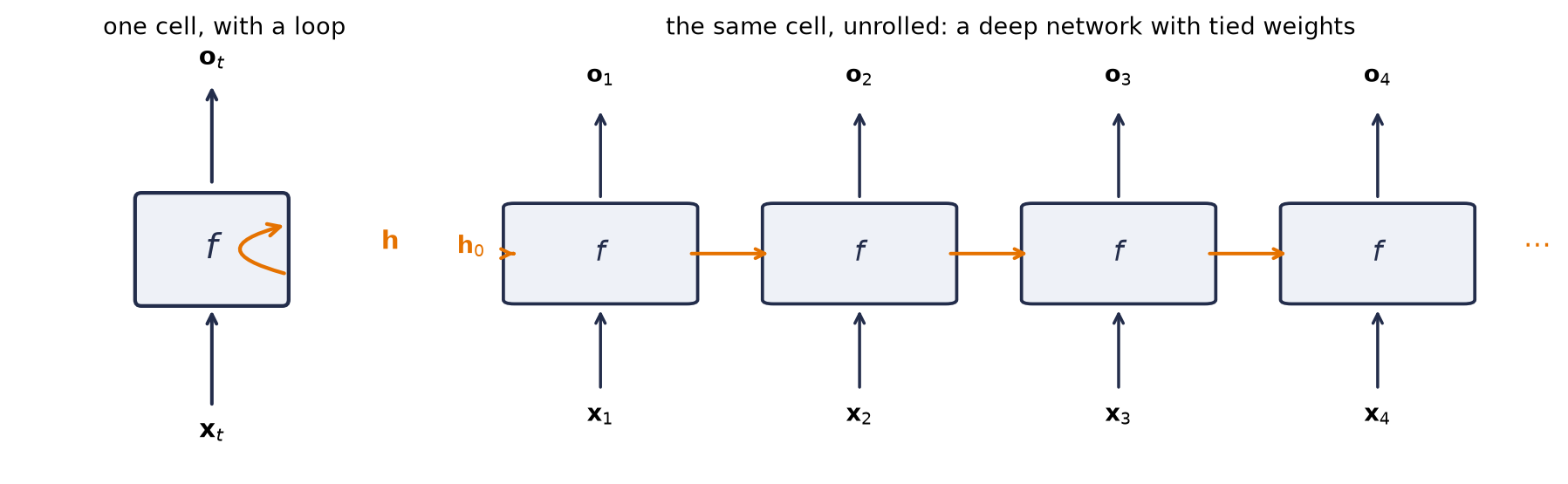
Unroll the loop on paper and the RNN is an ordinary feedforward network that happens to be \(T\) layers deep with every layer’s weights tied.
Figure 12.1: Two drawings of the same machine. Left: one cell whose hidden state loops back into itself. Right: the loop unrolled: a chain of copies of the same cell, each consuming one input and passing the state along. Read vertically it is an ordinary feedforward network; read horizontally it is a network as deep as the sequence is long, with every layer’s weights tied.
12.3 Gradients through time
The unrolled network is a deep network with tied weights, so backpropagation applies unchanged. Training on a sequence runs the loop forward, collects losses \(L_t\) at the readouts and sums them into \(L\), then backpropagates through the unrolled network, a procedure called backpropagation through time (BPTT). A gradient that lands on \(\vect{h}_T\) must travel back through every application of Equation 12.2 to reach an early input. Define \(\matr{D}_t = \mathrm{diag}\!\left(\tanh'(\cdot)\right)\) at step \(t\). The forward Jacobian for one hop is \(\matr{D}_t\matr{W}_{hh}\), so the full Jacobian is
The Jacobian is a product of \(T-1\) near-identical matrices. The second expression applies the chain rule in reverse-mode order to the adjoint \(\vect{g}_t=\partial L/\partial\vect{h}_t\), starting from \(\vect{g}_T=\partial L_T/\partial\vect{h}_T\) and ending at \(\vect{g}_0=\matr{W}_{hh}^{\!\top}\matr{D}_1\vect{g}_1\), since no loss is attached to \(\vect{h}_0\): the activation derivative \(\matr{D}_t\) scales the incoming gradient, \(\matr{W}_{hh}^{\top}\) carries it to the previous state, and the loss \(L_{t-1}\) adds its own gradient there.
A deep network’s gradient has the same form, a product of per-layer Jacobians. If the factors shrink the signal, the product decays exponentially; if they grow it, it explodes exponentially. Since \(\tanh' \le 1\) and \(\matr{W}_{hh}\) repeats at every step, keeping every relevant direction near unit gain over a long sequence is a fragile special case. Initialization can at least start there: an orthogonal \(\matr{W}_{hh}\) has every singular value equal to one, so wherever the pre-activations sit near zero, where \(\tanh'\approx 1\), each hop preserves the gradient’s norm. Training moves \(\matr{W}_{hh}\), and \(\tanh'\) drops below one as pre-activations grow, so orthogonality governs only the start of training (Exercise 2).
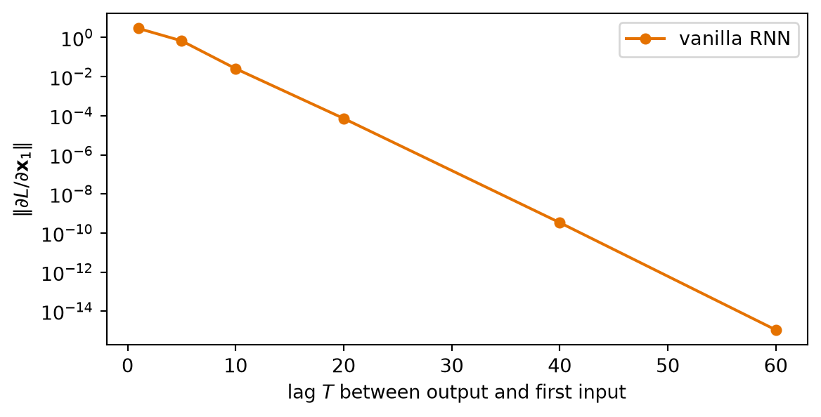
Earlier chapters measured depth in layers; here we measure it in time, and a paragraph of text, read one word per step, is about a hundred layers deep. We illustrate the effect of this depth in Figure 12.2, which plots, for a freshly initialized vanilla RNN, the norm of the gradient that reaches the first input against the lag \(T\), the length of the sequence (the first input lies \(T-1\) steps before the last).
Define the reusable grad_at_first_input helper.
Build a seeded vanilla nn.RNN and compute g_rnn at lags 1, 5, 10, 20, 40, and 60.
Gradient reaching the first input vs. lag.
# [1]def grad_at_first_input(rec: nn.Module, lags: list[int], vocab: int=4) ->list[float]: norms = []for T in lags: generator = torch.Generator().manual_seed(100+ T) x = torch.randn(8, T, vocab, generator=generator, requires_grad=True) o, _ = rec(x) o[:, -1].sum().backward() norms.append(x.grad[:, 0].norm().item()) # gradient at input #1return norms# [2]lags = [1, 5, 10, 20, 40, 60]torch.manual_seed(0)vanilla = nn.RNN(4, 32, batch_first=True)g_rnn = grad_at_first_input(vanilla, lags)# [3]print("lag: "+" ".join(f"{l:>7d}"for l in lags))print("|grad|: "+" ".join(f"{g:.1e}"for g in g_rnn))plt.figure(figsize=(6.2, 3.2))plt.semilogy(lags, g_rnn, "o-", color="#E57200", ms=5, label="vanilla RNN")plt.xlabel("lag $T$ between output and first input")plt.ylabel(r"$\|\partial L / \partial \mathbf{x}_1\|$")plt.legend(); plt.tight_layout(); plt.show()
Figure 12.2: Norm of the gradient \(\partial L/\partial\vect{x}_1\) that reaches the first input of a freshly initialized vanilla RNN, against the lag \(T\), the length of the sequence (the first input lies \(T-1\) steps before the last). Here \(L\) is the sum of the entries of the last state \(\vect{h}_T\) over the batch and the hidden units. The norm falls by about fifteen orders of magnitude from lag 1 to lag 60.
By lag 60 the gradient reaching the first input is about \(10^{-15}\): at initialization, whatever happened at the start supplies almost no usable learning signal. That makes success fragile rather than mathematically impossible. The mirror-image failure, explosion, is just as real: one large spike in Equation 12.4’s product can make an update destabilize training.
WarningGradient clipping limits explosion, not vanishing
In practice, explosion is handled with gradient clipping: if the gradient’s norm exceeds a threshold, it is rescaled down to the threshold before the step (nn.utils.clip_grad_norm_; it appears in every training loop below). This tames the spikes so training survives, at the cost of damping legitimately large steps. It does nothing for vanishing gradients, so clipping alone cannot lengthen the memory a recurrent network learns.
Training with a finite horizon
Full BPTT requires memory and compute for the entire sequence at each training update. The standard fix relies on the Markov property of the forward pass: the carried state and the next input together determine the next state. In truncated BPTT, contiguous chunks carry the recurrent state forward but detach it at each boundary. The values cross the boundary; the gradient graph does not. This bounds memory while preserving running context. For a cut after step \(t\), the next state is \[
\vect{h}_{t+1} = f\bigl(\operatorname{detach}(\vect{h}_t),\, \vect{x}_{t+1}\bigr),
\] where \(\operatorname{detach}\) returns the value of \(\vect{h}_t\) unchanged and passes no gradient back through it.
Where to cut is itself a choice: every \(K\) steps (a fixed horizon) or at random points. With a fixed horizon, the carried state still delivers the distant past to the forward pass, but the gradient trains only the dependencies whose two ends fall inside one chunk of \(K\) steps. A dependency that reaches \(\ell\) steps back links the loss at step \(t\) to the input at step \(t-\ell\). The loss at the \(j\)th step of a chunk reaches back \(j-1\) steps: just after a boundary (\(j=1\)) it reaches only its own input, and at the end of the chunk (\(j=K\)) it reaches back \(K-1\) steps. Only the losses at chunk steps \(\ell+1,\dots,K\), that is, \(K-\ell\) of the chunk’s \(K\) losses, therefore reach an input \(\ell\) steps back: such a dependency gets gradient from a fraction \(1-\ell/K\) of the losses, and from none once \(\ell \ge K\). With \(K=3\) and a cut after step 3, for example, the loss \(L_6\) uses the value that entered at \(\vect{x}_2\), four steps back; since \(4 \ge K\), no gradient from \(L_6\) reaches step 2. The model can use a longer dependency that its state happens to carry, but no gradient teaches it to keep one: a fixed horizon biases training toward short-range structure.
Random cuts alone do not remove the bias, because long-range terms are still the ones most often cut. Dividing each surviving gradient term by the probability that the cuts spared it does remove it: a term kept with probability \(p\) and scaled by \(1/p\) contributes its full value on average, so the estimate of the full gradient is unbiased (Tallec & Ollivier, 2017). The unbiased estimate has two costs: the rare long-range terms that survive arrive multiplied by large factors \(1/p\), which adds variance, and the number of steps whose activations must be stored varies from one update to the next. A fixed horizon stores activations for the same \(K\) steps in every update and adds no reweighting variance. Most training therefore keeps the fixed horizon, at the price of its bias.
The character model later in this chapter uses a simpler finite-horizon recipe: it samples random 100-character windows and starts each from zero state. That is fixed-window training, not truncated BPTT, because no state is carried between windows. It is cheap and appropriate for this small demonstration. In production character models, contiguous chunks of roughly 20–50 steps with carried-and-detached state are common. In either recipe, clipping handles spikes; neither creates gradients beyond the truncation horizon.
Watch the mechanism: what crosses a truncation cut
Two lanes train on the same six-step stream, cut into chunks of three. One carries the state across the cut, detached; the other resets it to zero. What crosses the cut in each lane: the value going forward, the gradient coming back, both, or neither?
A schematic of the two finite-horizon recipes just described: truncated BPTT carries the state across each cut and detaches it there; fixed-window training starts every window from zero state.
The values cross the boundary; the gradient graph does not.
0:00 / 0:40
The calculation is readable without playback. Opening this panel loads the optional controls.
Inside a chunk the gradient still flows back and still trains the shared weights; the cut removes only the paths that cross it.
Scope and caveats
Six steps and one cut after the third are a schematic. The recipes above carry and detach the state across chunks of roughly 20 to 50 steps, or sample 100-character windows that each start from zero state; neither length is drawn here.
In code, the carry lane is h = h.detach() between chunks, and the reset lane starts each window from a zero state.
Cutting at random points and dividing each surviving term by the probability that the cuts spared it, the unbiased alternative mentioned above, is not drawn. Clipping is a separate tool: it rescales large gradients and moves no cut.
Blue marks the carried value, wine the loss, its gradient and the rings on the states the gradient reaches, and ink the cut, the detach tag with its forward point, the zero start and the stop bar; the cells are grey. Shape and text carry the same distinctions: the value is a round packet on the line of states, the gradient a pointed packet on the rail beneath it.
Check yourself. Chunks of three steps, carried and detached, run for nine steps. The loss at step 9 depends on steps 5 and 7. Which of the two can its gradient reach?
Step 7, yes; step 5, no. The cuts fall after steps 3, 6 and 9, so steps 7, 8 and 9 share one chunk and the gradient of step 9's loss stops at the cut after step 6. Step 5's value still reaches step 9 through the carried state.
Transcript and keyboard help
Two lanes run the same stream of six steps, cut after step 3. The upper lane carries the state across the cut through a detach tag; the lower lane starts step 4 again from a zero box. Step 2's input is marked. Before playing on: what crosses the cut in each lane, the value going forward, the gradient coming back, both, or neither?
Step 2's input enters the state and rides to step 3 in both lanes, then holds there.
In the carry lane the value passes through the detach tag, crosses the cut and rides on to step 6; the states it reaches are shaded. In the reset lane it halts at the cut and fades to a ring, and step 4 starts again from zero.
The loss at step 6 appears in both lanes. Before playing on: how far back does its gradient travel in each lane?
The gradient runs back along the rail under the states, through steps 6, 5 and 4 in both lanes, and stops at the cut, where a short bar ends it. Each state it reaches wears a wine ring; steps 1 to 3 get none.
At the cut, the carry lane reads “value crosses” and “gradient stops”; the reset lane reads “value stops” and “gradient stops”. Detach passes the value but not the gradient; reset passes neither. The detach tag gains a forward point: a one-way gate.
The carry lane alone: step 6 uses step 2's value, carried through the cut, yet the gradient of step 6's loss stops at the cut and never reaches step 3 or step 2, so it cannot teach the model to keep that value.
The values cross the boundary; the gradient graph does not.
Silent; paused initially; 1.5× playback. Focus the animation pane: Space or K plays/pauses, arrows seek between beats, Home/End jump, Escape pauses. The scrubber and speed menu also work by keyboard. Reduced-motion mode holds each beat's finished state instead of moving between them.
12.4 Engineering a memory: the LSTM
In the vanilla RNN, the carried state passes through a weight matrix and a \(\tanh\) at every step, and its gradient through the repeated product of Equation 12.4. We can start with the additive update of residual networks and add multiplicative gates that control what the carried state keeps. We want a memory pathway that is:
Additive. Repeated multiplication attenuated the signal \(\rightarrow\) update the carried state additively: \(\vect{c}_t = \vect{c}_{t-1} + \vect{\Delta}_t\). This is the form of the residual connection, \(H(x) = F(x) + x\), whose Jacobian contains an identity term, now applied across time. How much of the state survives many steps depends on the gates below.
Forgettable on command. Some stored content should expire. A forget gate \(\vect{f}_t \in (0,1)\) multiplies \(\vect{c}_{t-1}\) elementwise.
Writable on command. New information enters through an input gate \(\vect{i}_t\) scaling a candidate \(\tilde{\vect{c}}_t\).
Readable on command. Expose only what the current step needs, through an output gate \(\vect{o}_t\).
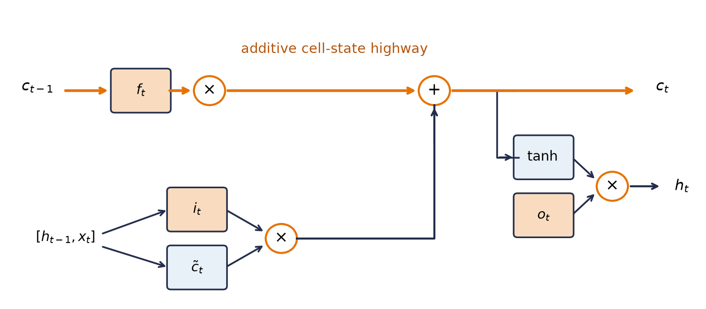
Each gate is a small learned layer squashed by a sigmoid (a number in \((0,1)\) read as what fraction passes). The candidate content is shaped by \(\tanh\), keeping it bounded and centered. Assembled, this is the Long Short-Term Memory cell (Hochreiter & Schmidhuber, 1997; the forget gate \(\vect{f}_t\) was added by Gers, Schmidhuber & Cummins, 2000):
Figure 12.3: The LSTM cell. All four learned layers read the same input \([h_{t-1}, x_t]\), drawn along the bottom. Along the top, the cell-state update path multiplies the old cell state elementwise by the forget gate \(f_t\) and adds the candidate content \(\tilde{c}_t\) scaled by the input gate \(i_t\); the output gate \(o_t\) controls what becomes visible as \(h_t\).
Watch the mechanism: close the output gate and look at the cell state
Close the output gate (ot → 0): is the memory erased?
This is the cell drawn just above, the LSTM update equations running once: the cell-state path carries c from the previous step through the forget gate, picks up the gated candidate at the sum, and leaves as c_t; a tanh branch through the output gate produces h_t. The chapter prints no gate values, so the three openings shown here are illustrative: each gate only ever stands at 1.0, 0.5 or 0.0, and the carried numbers (ct−1 = 1.00, the candidate 0.50) are round numbers chosen to be read, not measured. Every value on the picture is recomputed from them by the chapter's own two update lines.
The gates are learned; the cell state is not erased by closing the output gate.
0:00 / 0:40
The calculation is readable without playback. Opening this panel loads the optional controls.
The three openings are illustrative, not measured: the chapter prints no gate values here, and this panel stands each gate at 1.0, 0.5 or 0.0 so the arithmetic can be read off the picture.
Scope and caveats
Real gates are vectors, differ per unit and per step, and are produced by the sigmoid layers of the LSTM update equations from [h_{t−1}, x_t], which this panel does not evaluate. The chapter does measure gates once, later: its forget-gate diagnostic reports mean activations of about 0.76 for the task-solving model and about 0.56 for the default-initialized one, over eighty steps on sixty-four probe sequences. Those are measurements of two trained models, not the openings shown here, and they appear nowhere on the picture. Nothing here is trained and no gradient is drawn: the direct cell-state product of forget gates, the positive forget-gate bias, and the recall experiment are the chapter's next argument, and the GRU is out of scope.
Check yourself. Keep the picture's cell at 1.00 and now open the output gate fully. What is h?
h = 1 × tanh(1.00) ≈ 0.762, and the cell still holds 1.00. Reading passes the memory through tanh and the output gate; it does not spend it.
Transcript and keyboard help
The cell-state path runs left to right. The previous cell state stands on it at the inlet, 1.00 high. Before playing on: if the output gate is shut, is what the cell state carries lost?
Three gates appear, each drawn as a port with a vane: forget on the cell-state path, input on the branch that carries the candidate 0.50, output on the branch that leaves through tanh. Forget stands wide open at 1.00, input and output shut at 0.00, so the carried value crosses the forget gate untouched and parks mid-path at 1.00.
The forget gate closes halfway, to 0.50. The carried bar downstream of it halves in place: 1.00 becomes 0.50. Nothing else moved.
The input gate opens to 1.00. The candidate 0.50 travels up the branch into the sum, and the carried bar crosses the sum and grows to 1.00 at the outlet: 0.50 of old content plus 0.50 of new.
The output gate opens halfway, to 0.50. The branch through tanh lights and the hidden state rises to 0.38, half of tanh(1.00).
The output gate shuts to 0.00. The hidden state falls to 0.00, with a dashed mark left where it stood. The cell state's bar does not move: the cell state is still 1.00. Closing the output gate hides the memory; it does not erase it.
The two states are named: the cell state 1.00, long-term memory carried along the cell-state path, and the hidden state 0.00, the working memory the rest of the network sees.
A tag records that the three gates are not knobs: the weight matrices behind them are learned.
Silent; paused initially; 1.5× playback. Focus the animation pane: Space or K plays/pauses, arrows seek between beats, Home/End jump, Escape pauses. The scrubber and speed menu also work by keyboard. Reduced-motion mode holds each beat’s state: every gate stands at its beat’s opening, the carried bar stands at its beat’s station, and nothing is between two values.
Two states now travel: the cell state \(\vect{c}_t\) (long-term memory, carried along the cell-state path) and the hidden state \(\vect{h}_t\) (working memory, playing the vanilla RNN’s old role).
Let \(\vect{\gamma}_t := \partial L/\partial\vect{c}_t\) denote the loss sensitivity at the cell-state node. In the LSTM of Equation 12.5, the gates depend on \(\vect{h}_{t-1}\) and \(\vect{x}_t\), not directly on \(\vect{c}_{t-1}\). Holding the previous hidden state and the current input fixed, the direct cell-state Jacobian is diagonal. The contribution propagated from \(\vect{\gamma}_t\) along this path for \(k\) steps is
The product is elementwise. Forget-gate values near one reduce attenuation along this direct path. The full gradient also includes paths through hidden states, candidate updates, and gates; the displayed contribution is not the complete recurrent Jacobian. A positive forget-gate bias increases retention at initialization, all other gate inputs held fixed. The experiments below test how this choice affects training.
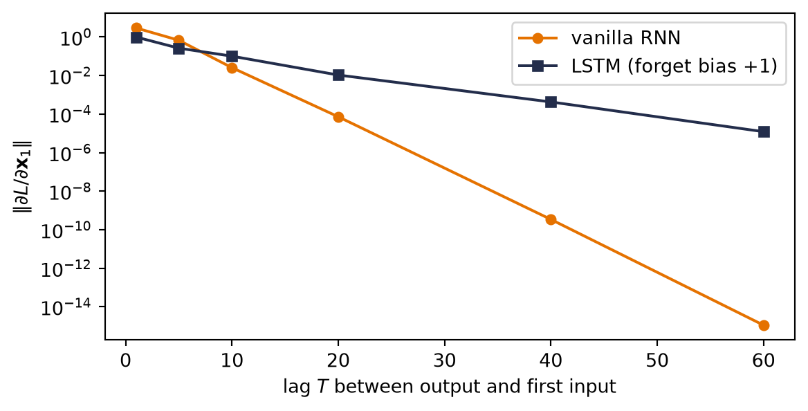
PyTorch stores separate input-hidden and hidden-hidden bias vectors, then adds them. The code sets their sum to \(+1\); setting both slices to \(+1\) would silently create an effective bias of \(+2\). Figure 12.4 repeats the measurement of Figure 12.2 for this LSTM: at lag 60 its input gradient is about ten orders of magnitude larger than the vanilla RNN’s.
Build a seeded nn.LSTM and set its two forget-gate bias slices to sum to +1.
Measure the LSTM gradient norm across lag.
# [1]torch.manual_seed(0)lstm = nn.LSTM(4, 32, batch_first=True)with torch.no_grad(): n = lstm.bias_ih_l0.shape[0] //4 lstm.bias_ih_l0[n:2* n].fill_(1.0) lstm.bias_hh_l0[n:2* n].zero_() # the two bias slices sum to +1# [2]g_lstm = grad_at_first_input(lstm, lags)
Figure 12.4: The gradient-vs-lag experiment of Figure 12.2, rerun on the same input sequences with an LSTM of the same size (4 inputs, 32 hidden units) whose effective forget-gate bias is initialized to +1. The vanilla RNN’s input gradient decays exponentially with the lag; the LSTM’s decays much more slowly and arrives at lag 60 attenuated, about ten orders of magnitude stronger.
Watch the mechanism: one word, eighty forget gates
A word enters at step 1 — how much of its gradient reaches step 80?
The cell-chain equation just above writes the contribution along the direct cell-state path as a product of forget gates, one per step. This panel holds one gate value f fixed for all 80 steps, which turns that product into a single power fk; the constant gate is this panel's simplification, not a claim of the chapter. It follows one word, cat, from step 1 to step 80 under two settings of the forget-gate bias bf. The chart and the two bands under it show the same number twice: as a curve and as ink. The slider is the one control; the timeline moves it first, and you may drag it after.
Sixteen trillion times larger, yet 10⁻¹¹ of the gradient: attenuated, not exactly zero. Legible only on a log axis.
0:00 / 0:40
The calculation is readable without playback. Opening this panel loads the optional controls.
A real forget gate is a vector, recomputed at every step from that step's input and state: it varies from unit to unit and from step to step.
Scope and caveats
The chapter's cell-chain equation gives only the direct cell-state contribution, with the previous hidden state and the input held fixed; the full gradient also follows paths through hidden states and gates. This panel simplifies further on purpose: one constant f, multiplied 80 times. Nothing here is trained, and nothing here is a claim about training. The two default gate values are σ(0) and σ(1), read off the sigmoid. The log axis has a floor of 10⁻²⁵, and in log mode a band's ink is 1 + log₁₀(fk)/25, clipped to [0, 1]: a word still legible at step 80 on the bf = +1 band is legible on that mapping, not intact — its gradient is about 10¹¹ times smaller than it was, attenuated, not exactly zero. The figure above measures something else: the norm of the gradient at lag 60, at initialization, for this LSTM against a vanilla RNN, which “arrives at lag 60 attenuated, about ten orders of magnitude stronger”: a measured quantity that is not this fk and is not reproduced here. What a trained network's gates actually do is the chapter's diagnostic, means near 0.76 for the solver and 0.56 for the default twin, over units and probes, for one task and one seed each. What shows that the bias matters is the chapter's recall experiment — 24% / 26% / 26% for the default LSTM against 100% / 100% / 100% with the forget bias at +1 — and that experiment, not this arithmetic, remains the chapter's evidence.
Check yourself. Suppose the forget gate sat at f = 0.9 on every step. What fraction of step 1's gradient reaches step 80?
About 2.18 × 10⁻⁴. Still attenuated — but some twenty orders of magnitude more than 0.5⁸⁰ ≈ 8.27 × 10⁻²⁵. Small changes in a gate that is multiplied eighty times are enormous changes in what survives.
Transcript and keyboard help
One chart of fk against the step k, empty; under it two bands, one per forget-gate bias, both white, with the word cat waiting at step 1 on each; the bf slider at 0. Before it moves, answer for yourself: how much of the word's gradient reaches step 80?
bf = 0, so every gate is σ(0) = 0.500. The word travels the upper band; the dashed curve is its trace, and the band's ink at step k is 0.5k itself. By step 8 the ink is below a screen's least tint and the word has become · · ·; by step twelve the gradient is 2.44 × 10⁻⁴ of what entered.
The slider slides to bf = +1: every gate is now σ(1) = 0.731. The word travels the lower band and the solid curve traces it. On a linear axis this curve also plunges: by step twenty the ink is 0.73120 = 1.90 × 10⁻³, and both bands look dead.
The axis switches to log, floor 10⁻²⁵, and the bands re-map: ink is now 1 + log₁₀(fk)/25, clipped to [0, 1]. The two curves straighten into lines of slope −0.301 and −0.136 per step; the upper band fades to nothing exactly at step 80, the lower keeps a clear tint all the way.
Arrival. At step 80 the dashed curve reads 8.27 × 10⁻²⁵, about 10⁻²⁴, the value Appendix A3 prints for a forget gate at its default initialization, and the solid curve 1.31 × 10⁻¹¹. The badge between them is their ratio, × 1.6 × 10¹³: sixteen trillion times larger. The word on the upper band is · · ·; on the lower it is a faint but legible cat, legible on the log mapping only: its gradient is 10⁻¹¹ of what entered, attenuated, not exactly zero.
The slider sweeps to +2 and back. At +2 every gate is σ(2) = 0.881, step 80 reads 3.89 × 10⁻⁵ and the badge × 4.7 × 10¹⁹, forty-seven quintillion times larger; the lower band, its word and the solid curve follow, the dashed curve and the upper band do not. The slider's other ticks: −1 gives σ(−1) = 0.269 and 2.36 × 10⁻⁴⁶; −2 gives σ(−2) = 0.119 and 1.27 × 10⁻⁷⁴. Drag bf yourself: the gate's resting value decides what survives.
Hold at bf = +1: 8.27 × 10⁻²⁵ against 1.31 × 10⁻¹¹, sixteen trillion times larger, yet 10⁻¹¹ of the gradient.
Silent; paused initially; 1.5× playback. Focus the animation pane: Space or K plays/pauses, arrows seek between beats, Home/End jump, Escape pauses. The scrubber and speed menu also work by keyboard. The bf slider is the one parameter control: the timeline moves it, and dragging it pauses playback and recomputes the whole picture from the dragged value; its arrow keys move bf by 0.05 and never seek the timeline, and Play resumes the timeline's own bf. The linear/log switch is available from the log beat on and whenever playback is paused. Reduced-motion mode holds each beat's state: the word jumps to each beat's end position, the slider to each beat's value (+2 for the sweep beat), the axis to the beat's mode.
12.5 GRU: gating with one state
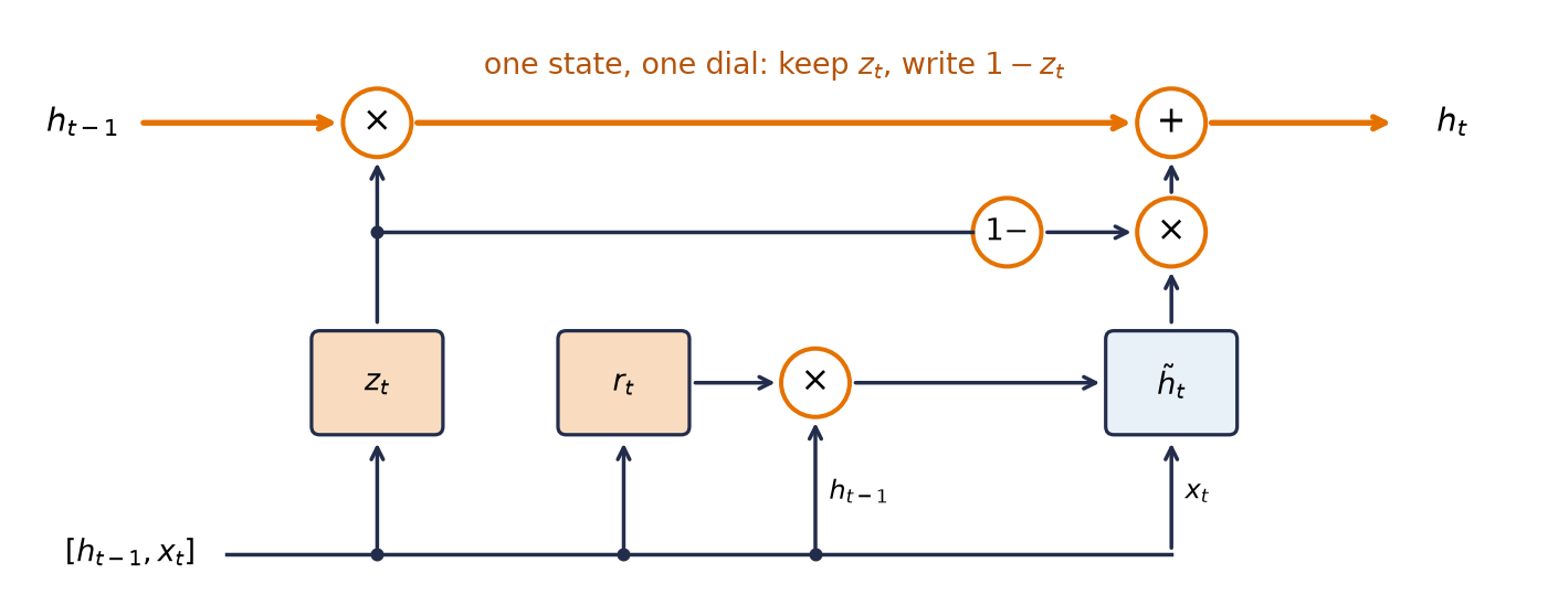
The Gated Recurrent Unit (Cho et al., 2014) folds the same ideas into a smaller box: cell and hidden state merged into one \(\vect{h}_t\), forget and input gates merged into a single update gate\(\vect{z}_t\) (what you keep you do not overwrite, and vice versa), plus a reset gate\(\vect{r}_t\) that can blank the past when a fresh start is called for:
This follows Cho et al.’s original convention: \(\vect{z}_t\) weights the old state, so it reads as keep. Some later references reverse the symbol and let \(\vect{z}_t\) weight the candidate instead; compare the interpolation equation, not the gate’s name alone.
The GRU has two gates instead of three and one state instead of two, and in most settings its performance is comparable to the LSTM’s. The memory test below puts PyTorch’s version beside the LSTM, and Exercise 3 builds one by hand. Figure 12.5 draws the cell on the layout of Figure 12.3.
Figure 12.5: The GRU cell on the LSTM cell’s layout. One state travels: the update gate \(z_t\) keeps a fraction of \(h_{t-1}\), and the same dial’s complement \(1 - z_t\) writes in the candidate \(\tilde{h}_t\). The reset gate \(r_t\) scales \(h_{t-1}\) before the candidate reads it, as in Equation 12.7.
Watch the mechanism: halve the keep gate and follow the new state
One coordinate of the state holds 0.80, and the candidate offers 0.30. With the keep gate fully open, the new state stays at 0.80. Halve the keep to 0.5: where does the new state land?
One coordinate of the cell drawn above: the old state and the candidate on a line from −1 to 1, and the keep gate as a dial.
One dial, two jobs: keep z of the old state, write 1 − z of the candidate.
0:00 / 0:40
The calculation is readable without playback. Opening this panel loads the optional controls.
The values 0.80 and 0.30 are an illustrative toy: a real cell gives every coordinate its own keep, computed by a sigmoid from the input and the old state.
Scope and caveats
The two values are round numbers inside the range of tanh, which shapes every candidate; the chapter trains its gates and prints no state values. A real state is a vector, and every coordinate of \( \vect{z}_t \) is a keep of its own, so one coordinate can hold its value while its neighbor is overwritten.
The reset gate decides how much of the old state the candidate reads: it shapes the candidate before the blend and is not drawn. PyTorch’s reset-after candidate changes how the candidate is computed, not this blend.
This panel follows the chapter’s convention: \( \vect{z}_t \) weights the old state, so it reads as keep. Some references swap the roles; compare the interpolation equation, not the gate’s name.
Blue marks every value the cell carries: the filled circle is the old state, the hollow diamond the candidate, the ring the new state, and the arrows their kept and written shares, filled and hollow like the marks they come from. The keep and write bar and the dial are neutral ink: a gate weighs values and carries none. The bar puts write on the left and keep on the right, the sides where the candidate and the old state sit on the line and where the dial writes all or keeps all, and each share is named beside its value's mark.
Check yourself. A GRU starts from h0 = 0, and every candidate it writes is a tanh output inside (−1, 1). Can a coordinate of its state ever reach 1.2, whatever the gates do?
No. Each step lands the new state on the segment between the old state and the candidate, since keep and write are shares of one whole. If both ends lie inside (−1, 1), so does the new state, and from h0 = 0 every state stays inside (−1, 1).
Transcript and keyboard help
A number line from −1 to 1, the range of tanh. The old state sits at 0.80, a filled circle; the candidate at 0.30, a hollow diamond. The keep gate is fully open, so the bar is all keep and the new state, a ring, sits under the old state at 0.80.
The keep halves to 0.5: the bar splits into write on the left and keep on the right, half each, and the new state leaves the picture. Predict: where does it land?
The old state becomes an arrow from 0 to 0.80, and the keep shrinks it to half: 0.5 × 0.80 = 0.40.
The candidate becomes an arrow from 0 to 0.30. What is not kept is written: it shrinks to 0.5 × 0.30 = 0.15 and slides onto the tip of the kept arrow, and the new state lands at that tip, 0.40 + 0.15 = 0.55.
The segment from the candidate to the old state is marked. With equal shares, 0.55 sits halfway along it.
The dial turns up to full keep. The kept arrow grows back to 0.80, the written arrow shrinks to nothing, and the new state slides along the segment to 0.80.
The dial turns down to keep 0. The kept arrow shrinks to nothing and the written arrow carries the whole candidate: the new state slides the length of the segment to 0.30, overwritten.
Home at keep 0.5: 0.40 kept plus 0.15 written gives 0.55. One dial does two jobs, keeping z of the old state and writing 1 − z of the candidate, so the new state always lands on the segment between them. Drag the dial to try another keep.
Silent; paused initially; 1.5× playback. Focus the animation pane: Space or K plays/pauses, arrows seek between beats, Home/End jump, Escape pauses. The scrubber and speed menu also work by keyboard. The keep dial pauses playback and redraws the whole picture for the keep you choose; playing or scrubbing returns to the timeline. Reduced-motion mode holds each beat’s finished state instead of moving between them.
One convention matters before you compare code. Equation 12.7 applies the reset gate to \(\vect{h}_{t-1}\)before the candidate’s hidden-state linear map. PyTorch’s nn.GRU uses a reset-after form, \(\tanh(\matr{W}_{in}\vect{x}_t + \vect{b}_{in} + \vect{r}_t \odot (\matr{W}_{hn}\vect{h}_{t-1} + \vect{b}_{hn}))\), for implementation efficiency. The gates serve the same purpose, but the two cells are not algebraically identical for the same weights. An exact manual-loop verification must implement PyTorch’s ordering rather than Equation 12.7’s.
12.6 The memory test
We measured the gradients above at initialization; now we train. The task is a two-company story: Company A’s prices open at 0, Company B’s at 1, then both trade identically for days, and the correct day-5 prediction is whatever day 1 said. Solving it requires carrying one early bit across a long stretch of identical noise. As an executable task, the story becomes sequences of 80 random tokens, and the label to predict at the end is the first token. Chance is 25%. We compare six contenders, three seeds each: the vanilla RNN; the LSTM and the GRU with PyTorch’s default initialization; the LSTM with its forget-gate bias \(\vect{b}_f\) set to \(+1\) in every unit; and the GRU with its keep-gate bias \(\vect{b}_z\) set the same way, at \(+1\) and at \(+2\).1 Each row also reports its input-gradient norm at initialization: the norm of the gradient reaching the first input at lag 80, measured as in Figure 12.2 on the third run’s initialization, before any training. The printout below calls this norm the signal at birth. Predict the rows before running: is a gated architecture alone enough, and does the LSTM’s \(+1\) carry over to the GRU?
Define the reusable helpers: make_recall, SeqClassifier, and train_recall.
Set T = 80, list the vanilla RNN, two LSTM setups, and three GRU setups, make an empty probe_nets, and print a header.
Train every setup on three seeds; print its signal at birth and its accuracies.
# [1]def make_recall(n: int, T: int, vocab: int=4, seed: int=0) ->tuple[torch.Tensor, torch.Tensor]: g = torch.Generator().manual_seed(seed) X = torch.randint(0, vocab, (n, T), generator=g)return F.one_hot(X, vocab).float(), X[:, 0] # label = first tokenGATES = {"gru": 3, "lstm": 4} # gate slices stacked in a biasclass SeqClassifier(nn.Module):def__init__(self, cell: str, vocab=4, hidden=32, keep_bias=None):super().__init__()self.rec = {"rnn": nn.RNN, "gru": nn.GRU, "lstm": nn.LSTM}[cell]( vocab, hidden, batch_first=True)if keep_bias isnotNone: # LSTM forget gate, GRU update gatewith torch.no_grad(): n =self.rec.bias_ih_l0.shape[0] // GATES[cell]self.rec.bias_ih_l0[n:2* n].fill_(keep_bias)self.rec.bias_hh_l0[n:2* n].zero_()self.out = nn.Linear(hidden, vocab)def forward(self, x: torch.Tensor) -> torch.Tensor: o, _ =self.rec(x)returnself.out(o[:, -1]) # read out at the END onlydef train_recall(cell: str, T: int, seed: int, keep_bias: float|None=None, epochs: int=80) ->tuple[float, nn.Module, float]: torch.manual_seed(seed) net = SeqClassifier(cell, keep_bias=keep_bias) birth = grad_at_first_input(net.rec, [T])[0] # own generator: no RNG drawn X_tr, y_tr = make_recall(2000, T, seed=1) X_te, y_te = make_recall(500, T, seed=2) opt = torch.optim.Adam(net.parameters(), lr=3e-3)for _ inrange(epochs): perm = torch.randperm(len(X_tr))for i inrange(0, len(X_tr), 128): idx = perm[i:i +128] loss = F.cross_entropy(net(X_tr[idx]), y_tr[idx]) opt.zero_grad(); loss.backward() nn.utils.clip_grad_norm_(net.parameters(), 1.0) opt.step()with torch.no_grad(): acc = (net(X_te).argmax(1) == y_te).float().mean().item()return acc, net, birth# [2]T =80configs = [("vanilla RNN", "rnn", None), ("LSTM, default init", "lstm", None), ("LSTM, forget bias +1", "lstm", 1.0), ("GRU, default init", "gru", None), ("GRU, keep bias +1", "gru", 1.0), ("GRU, keep bias +2", "gru", 2.0)]probe_nets: dict[str, nn.Module] = {} # kept for the diagnostic belowprint(f"recall at lag {T} (chance 25%): signal at birth (seed 6050), ""then accuracy for seeds 0 / 1 / 6050")# [3]for label, cell, kb in configs: results = [train_recall(cell, T, s, kb) for s in [0, 1, 6050]] accs = [a for a, _, _ in results] probe_nets[label] = results[-1][1] # seed 6050's modelprint(f" {label:22s}{results[-1][2]:8.1e} "+" ".join(f"{a:4.0%}"for a in accs))
Under this recipe, the LSTM with forget bias \(+1\) and the GRU with keep bias \(+2\) solve the task on all three tested seeds. The vanilla RNN solves it on one seed, while the remaining configurations stay near chance. The comparison shows that initialization materially affects the outcome in this task; gated architecture alone does not ensure successful training. In these tested configurations the GRU succeeds at \(+2\) but not at \(+1\). Its update gate both keeps the old state and admits the candidate in Equation 12.7, and equal bias settings in different cells do not imply equal realized gate values or recurrent Jacobians (Exercise 3 compares the two cells’ Jacobians).
The initial-gradient measurements use the initialization of the third run only. For that initialization, the two configurations that succeed on all three training seeds also have larger measured gradients at the first input.2 This is a diagnostic association in the reported experiment, not a general threshold for successful training.
Inspecting the forget gates
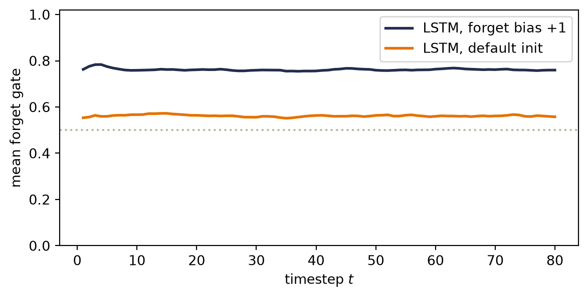
The recall results suggest a check on the gates themselves. If the forget-bias model retains the first token along the direct cell-state path of Equation 12.6 across the eighty-step gap, its mean forget gate should hold clearly above the half-open point, step after step, while the default model’s should stay near \(\sigma(0) = \tfrac12\). The default-initialized LSTM is the control: it has the same architecture, was trained on the same data, and scores at chance.
Define the reusable forget_gate_trace helper.
Open the figure for the forget-gate traces.
Replay the trained LSTMs and read their forget gates.
# [1]@torch.no_grad()def forget_gate_trace(net: SeqClassifier, T: int=80) ->list[float]: X_probe, _ = make_recall(64, T, seed=3) # fresh probe sequences lstm = net.rec W_ih, W_hh = lstm.weight_ih_l0, lstm.weight_hh_l0 b = lstm.bias_ih_l0 + lstm.bias_hh_l0 hidden = W_hh.shape[1] h = torch.zeros(64, hidden) c = torch.zeros(64, hidden) means = []for t inrange(T): # replayed by hand z = X_probe[:, t] @ W_ih.T + h @ W_hh.T + b i_gate, f_gate, g_cand, o_gate = z.chunk(4, dim=1) f = torch.sigmoid(f_gate) c = f * c + torch.sigmoid(i_gate) * torch.tanh(g_cand) h = torch.sigmoid(o_gate) * torch.tanh(c) means.append(f.mean().item()) out_ref, _ = lstm(X_probe) # replay must match the moduleassert torch.allclose(h, out_ref[:, -1], atol=1e-5)return means# [2]plt.figure(figsize=(6.2, 3.2))# [3]for label, color in [("LSTM, forget bias +1", "#232D4B"), ("LSTM, default init", "#E57200")]: plt.plot(range(1, T +1), forget_gate_trace(probe_nets[label]), color=color, lw=2, label=label)plt.axhline(0.5, ls=":", color="#B8B8A8", label=r"$\sigma(0) = \frac{1}{2}$")plt.ylim(0, 1.02)plt.xlabel("timestep $t$")plt.ylabel("mean forget gate")plt.legend(loc="lower right")plt.tight_layout(); plt.show()
Figure 12.6: Mean forget-gate activation per timestep on 64 fresh probe sequences, replayed through the two trained LSTMs of the third run in the table above. The task-solving model (navy) holds its gates flat around 0.76 for all eighty steps. The default-initialized model (orange), same architecture and data, stays near \(\sigma(0)\approx\tfrac12\) at about 0.56 and scores at chance.
The replay executes Equation 12.5 by hand with the trained weights, and an assertion confirms that it reproduces the module’s own output.
The forget-bias model’s higher mean forget gate is consistent with greater retention along the direct cell-state path. A mean over units and probes, however, does not identify which units retain the first token, nor does it measure the full recurrent sensitivity.
NoteHistorical bridge (optional): before contextual states
Word2Vec learned a fixed vector for each word type through local prediction: skip-gram predicts nearby words from a center word, while CBOW predicts the center from its neighborhood. GloVe used corpus-wide co-occurrence counts, fitting vector dot products and biases to their logarithmic structure. Both made distributional meaning learnable, but both returned a static lookup: the stored vector for bank did not change between a river and a loan.
The recurrent state in this chapter changes that contract. Its \(h_t\) depends on the visible prefix, so the representation at a position is contextual even when its input token embedding began as a lookup. Later we will build a different mechanism that lets each position mix information from other visible positions directly.
12.7 The book reads itself
We now apply fixed windows, clipping, gates, and a softmax over a vocabulary to real text. The task is the oldest one in language modeling: read a character, predict the next. The corpus is the markdown source of nine earlier chapters, Chapters 1 to 6 and 8 to 10, with the code cells removed. Its prose and LaTeX mathematics come to about 150,000 characters, kept as a fixed snapshot so that later copyedits cannot change the task.
Read the committed corpus book-corpus-ch1-9.txt into the string text.
Check the corpus snapshot, build the character vocabulary, and split the encoded text 90/10 into train_data and valid_data.
Print the corpus length and vocabulary size, then the train and held-out split sizes.
Define the CharLSTM module.
import hashlibfrom pathlib import Path# [1]corpus_path = Path("../../data/book-corpus-ch1-9.txt")text = corpus_path.read_text(encoding="utf-8")# [2]assertlen(text) ==148_594assert hashlib.sha256(text.encode("utf-8")).hexdigest() == ("b0fc23a513e37e7bcd78da04a03877345f6ebc850b91dbae260656d9924fb299")chars =sorted(set(text))stoi = {c: i for i, c inenumerate(chars)}data = torch.tensor([stoi[c] for c in text])split =int(0.9*len(data))train_data, valid_data = data[:split], data[split:]# [3]print(f"corpus: 9 chapters, {len(text):,} characters, vocab {len(chars)}")print(f"deterministic split: {len(train_data):,} train / {len(valid_data):,} held out")# [4]class CharLSTM(nn.Module):def__init__(self, vocab: int, hidden: int=128):super().__init__()self.vocab = vocabself.lstm = nn.LSTM(vocab, hidden, batch_first=True)self.out = nn.Linear(hidden, vocab)def forward(self, x: torch.Tensor, state: tuple[torch.Tensor, torch.Tensor] |None=None, ) ->tuple[torch.Tensor, tuple[torch.Tensor, torch.Tensor]]: o, state =self.lstm(F.one_hot(x, self.vocab).float(), state)returnself.out(o), state # logits at EVERY step
corpus: 9 chapters, 148,594 characters, vocab 104
deterministic split: 133,734 train / 14,860 held out
The training loop below is the canonical next-token trainer: Listing 12.1. Each update samples fresh random 100-character windows and clips the gradient; each window starts from zero state, as in fixed-window training. Because the state is reset, the window also caps the context length at 100 characters, in training and in the fixed-window evaluation below: a limit of the recipe, not of the LSTM. The listing is included from tested source in the support module (code/dlbook/training.py), and the cell after it imports and runs that same file.
Listing 12.1: the canonical next-token trainer:
Declare the shared next-token training interface and its protocol controls.
Configure the optimizer and requested step budget.
Draw or reuse chunk starts, then construct shifted input–target pairs.
Predict every next token and average cross-entropy across batch and time.
Backpropagate, clip the gradient, and take one optimizer step.
Retain a sparse learning curve and return the trained artifact.
"""Next-token training loop — Chapter 12's listing, importable.The loop is printed and taught in Chapter 12 (fixed-window chunk sampling,gradient clipping); later chapters import it and print only their deltas."""import torchimport torch.nn.functional as Ffrom torch import nn# [1]def fit_next_token( model: nn.Module, data: torch.Tensor,*, vocab: int, context: int=100, batch: int=64, steps: int=2501, lr: float=2e-3, clip: float=1.0, schedule: list[torch.Tensor] |None=None, log_every: int=500, log_decimals: int=2,) ->tuple[nn.Module, list[tuple[int, float]]]:"""Train `model` to predict data[t+1] from data[t-context+1 .. t]. With `schedule=None`, chunk starts are drawn fresh each step (Chapter 12's fixed-window sampling, consuming the global RNG exactly as printed there). A precomputed `schedule` of start tensors makes the minibatch order an explicit, shareable part of the protocol (Chapter 16's paired comparison). """# [2] opt = torch.optim.Adam(model.parameters(), lr=lr) curve: list[tuple[int, float]] = [] n_steps =len(schedule) if schedule isnotNoneelse steps# [3]for step inrange(n_steps): starts = ( schedule[step]if schedule isnotNoneelse torch.randint(0, len(data) - context -1, (batch,)) ) xb = torch.stack([data[j : j + context] for j in starts]) yb = torch.stack([data[j +1 : j + context +1] for j in starts])# [4] logits = model(xb)ifisinstance(logits, tuple): # recurrent models return state logits = logits[0] loss = F.cross_entropy(logits.reshape(-1, vocab), yb.reshape(-1))# [5] opt.zero_grad() loss.backward() nn.utils.clip_grad_norm_(model.parameters(), clip) opt.step()# [6]if step % log_every ==0: curve.append((step, loss.item()))print(f"step {step:4d} loss {loss.item():.{log_decimals}f}")return model, curve
Listing 12.2: the fixed-window evaluation protocol (state reset at every window boundary, so train and held-out numbers stay comparable across chapters):
Declare inference-only fixed-window evaluation.
Switch to evaluation mode and initialize token-weighted totals.
Traverse consecutive non-overlapping windows.
Predict with recurrent state reset at each window boundary.
Sum loss within windows and count all scored tokens.
Divide once to obtain mean next-token cross-entropy.
"""Fixed-window evaluation loss — Chapter 12's protocol, importable.Scores a sequence in consecutive `window`-sized chunks with the recurrent (orattention) state reset at each boundary, so train and held-out numbers arecomparable across chapters and architectures."""import torchimport torch.nn.functional as Ffrom torch import nn# [1]@torch.no_grad()def fixed_window_loss( net: nn.Module, sequence: torch.Tensor,*, vocab: int, window: int=100,) ->float:"""Mean next-token cross-entropy over non-overlapping windows."""# [2] net.eval() total_loss, n_tokens =0.0, 0# [3]for start inrange(0, len(sequence) -1, window): stop =min(start + window, len(sequence) -1) xb = sequence[start:stop].unsqueeze(0) yb = sequence[start +1 : stop +1]# [4] logits = net(xb)ifisinstance(logits, tuple): # recurrent models return state logits = logits[0] # state resets at each window# [5] total_loss += F.cross_entropy( logits.reshape(-1, vocab), yb, reduction="sum" ).item() n_tokens += yb.numel()# [6]return total_loss / n_tokens
Fix the seed and build a fresh CharLSTM sized to the corpus vocabulary.
Train it with fit_next_token (Listing 12.1).
Score the trained model on valid_data with fixed_window_loss and print the loss.
step    0   loss 4.62
step  500   loss 2.28
step 1000   loss 1.93
step 1500   loss 1.75
step 2000   loss 1.57
step 2500   loss 1.42
held-out fixed-window loss 1.89
The loss falls from the uniform-guessing value \(\ln(V) \approx 4.6\) for the printed vocabulary size to 1.42 on the last sampled training minibatch. The deterministic held-out tail is harder, at 1.89, but both are far below uniform guessing. To see what the model has learned, we generate text: we feed a prompt, divide the last step’s logits by a temperature\(\tau\), take the softmax, and sample the next character from the result; that character goes back in, and the loop repeats. A temperature below 1 sharpens the distribution, and as \(\tau \to 0\) each draw becomes the argmax; above 1 it flattens toward uniform. The sampler below uses \(\tau = 0.8\). The hidden state streams, so nothing is recomputed, and generation can run past the 100 characters of a training window, although no training loss depended on a longer context.
Define the reusable sample helper.
Sample from the model, one character at a time.
# [1]@torch.no_grad()def sample(prompt: str, n: int=300, temp: float=0.8) ->str: model.eval() idx = torch.tensor([[stoi.get(c, 0) for c in prompt]]) logits, state = model(idx) out = promptfor _ inrange(n): p = F.softmax(logits[0, -1] / temp, -1) nxt = torch.multinomial(p, 1)[None] out += chars[nxt.item()] logits, state = model(nxt, state) # consume each sample oncereturn out# [2]print(sample("The gradient ", n=300))
The gradient mupolition both
lates
chood each the burk's map into a mack from the bupfured way
   intene agmenten. Pyout nothing buith and why the dirge melies to exactly. What algien is

$$
\logit_i).
   ixsections.

## Exercise reseds the barkwarper from to twe optimized $\rightarrow$ and classitivations, in t
Trained on raw text in 100-character windows, the one-layer model has learned words, spacing, markdown furniture (headings, display-math dollar signs, backslashed macros), and the book’s working vocabulary (Exercise, map, optimized, and misspelled cousins). Clauses trail off, and equations open and never close: the sample reproduces local vocabulary and formatting but does not sustain coherent statements. This run does not separate the effects of corpus size, state width, training horizon, and optimization.
12.8 At full scale: words, layers, and corpus size
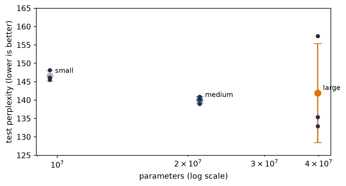
The character model answered the chapter’s mechanism question on a CPU-sized snapshot. It did not answer what happens when tokens become words, the corpus grows past two million training tokens, and recurrent depth increases. We ran that experiment on WikiText-2 with a 33,279-word training vocabulary. Three tied-embedding LSTMs share the same optimizer and 12-epoch budget; validation selects one checkpoint before the test split is opened.
Load the nine stored WikiText-2 run records.
Summarize parameter count and held-out perplexity by model size.
# [1]import jsonfrom pathlib import Pathwikitext_root = Path("../../experiments/rivanna/results/wikitext")wikitext_records = [ json.loads(path.read_text()) for path insorted(wikitext_root.glob("*.json"))]wikitext_order = ["small", "medium", "large"]# [2]wikitext_summary = {}for size in wikitext_order: rows = [row for row in wikitext_records if row["size"] == size] perplexities = torch.tensor([row["test_perplexity"] for row in rows]) wikitext_summary[size] = {"parameters": rows[0]["parameter_count"],"values": perplexities,"mean": perplexities.mean().item(),"sd": perplexities.std(unbiased=True).item(), }
Figure 12.7: Word-level LSTM scale on WikiText-2. Across three seeds, the 9.61M-parameter model reaches test perplexity 146.59 ± 1.38, the 21.27M model 140.05 ± 0.98, and the 39.77M model 141.94 ± 13.49. The medium model improves reliably; the largest has two strong runs and one poor run, so more parameters did not buy a stable improvement under the shared 12-epoch recipe. Points are seed-level tests; bars are means ± one sample standard deviation.
Moving from 9.61M to 21.27M parameters improves every seed. Moving again to 39.77M does not improve the mean reliably: two runs are strongest, while the third ends at perplexity 157.44. Capacity, optimization, and data must scale together.
12.9 What a single carried state does not provide
Against the six goals, the window met the first four and failed reach; a function per timestep failed two at once: any length and parameters independent of length. One shared recurrence met the first five on paper. On the sixth, at lag 80 on our task, the vanilla cell trained successfully on one of three seeds, while the LSTM with forget bias \(+1\) and the GRU with keep bias \(+2\) did so on all three tested seeds. Two needs outside the list remain.
The first is revisiting earlier evidence. In a recurrence, the input at step \(s\) reaches step \(t\) only through the \(t-s\) updates that follow it, the same chain that the gradient crosses backward in Equation 12.4. Suppose one recurrent network, an encoder, reads a source sentence, and a second, a decoder, starts from the encoder’s final state and writes a translation. Every source word then reaches the decoder through that one state, and the decoder has no direct access to earlier source positions. Revisiting requires keeping the whole sequence of states and computing, at each output step, how much to read from each.
The second is time in parallel. Every loop in this chapter runs one step at a time: \(\vect{h}_t\) cannot be computed before \(\vect{h}_{t-1}\), so a sequence’s length is also its training’s critical path. Two remedies exist: replace the recurrence with a mechanism that combines information from all positions at once, or keep a recurrence simple enough to compute in parallel (Exercise 8 builds the second in miniature).
NoteCheck yourself
Close the book for one minute and unroll the recurrence.
What is shared across timesteps, and what changes at each step?
How does an LSTM cell create a less obstructed path for information and gradients?
Which of the six goals does each design in this chapter fail, and what can a decoder initialized only from a final state not access directly?
12.10 Okay, so: weight sharing moved into time
Six streaming design goals: any length, order (in language a rearrangement can change the meaning), streaming, parameters independent of length, reach, and trainable reach. None of the fixed-size models built in Parts I–II meets all six.
Shared transition parameters: one update rule \(f\), with the same parameters at every timestep, carrying a hidden state (Equation 12.1, Equation 12.2). The rule is time-homogeneous, extending the sharing across space of Part II; its output can still depend on position through the state. The unrolled RNN is a deep network with tied weights.
Tied depth in time repeats the deep-network problem: BPTT multiplies \(T-1\) near-identical Jacobians (Equation 12.4) \(\rightarrow\) vanishing or exploding, unless their gains are carefully controlled. The recurrence gives computational reach to every earlier input, but a gradient must cross that product, and a finite training horizon supplies none across its boundary. Clipping tames the explosions; truncation caps the cost, but neither lengthens the range of dependencies that training can teach.
The LSTM engineers the memory: an additive cell-state update, the residual connection’s form applied across time, with three sigmoid gates (forget, input, output; Equation 12.5). Along the direct cell-state path, the gradient contribution is scaled by a product of forget gates, not weight matrices (Equation 12.6); the full gradient also follows paths through hidden states and gates.
Initialization affects recall: at lag 80 the default LSTM scores near chance; with the forget bias set to \(+1\) it solves the task on all three tested seeds. The GRU packs the same ideas into two gates and one state (Equation 12.7); in these tests it succeeded with keep bias \(+2\) but not \(+1\). At the one measured initialization, the two configurations that succeeded on all three seeds had the largest input-gradient norms: an association in this experiment, not a general threshold.
A one-layer character LSTM reproduces local features of this book (words, spacing, markdown and LaTeX markup) but does not sustain coherent statements; this experiment does not separate corpus size, state width, training horizon, and optimization. Two needs remain, revisiting and time in parallel: earlier inputs reach later steps only through one fixed-size state, so a decoder initialized from a final state has no direct access to earlier positions; and a loop must finish each step before starting the next.
Sources and further reading
Merity, S., Xiong, C., Bradbury, J., & Socher, R. (2017). Pointer Sentinel Mixture Models. International Conference on Learning Representations (ICLR 2017). arXiv:1609.07843. Introduces the WikiText corpora used by the chapter’s word-level language-model scale study.
Elman, J. L. (1990). Finding Structure in Time. Cognitive Science, 14(2), 179–211. The classic simple recurrent network and its view of hidden state as temporal context.
Hochreiter, S., & Schmidhuber, J. (1997). Long Short-Term Memory. Neural Computation, 9(8), 1735–1780. The original gated-memory architecture and constant-error pathway.
Gers, F. A., Schmidhuber, J., & Cummins, F. (2000). Learning to Forget: Continual Prediction with LSTM. Neural Computation, 12(10), 2451–2471. Adds the adaptive forget gate to the 1997 cell, giving the form used in this chapter.
Cho, K., van Merriënboer, B., Gulcehre, C., Bahdanau, D., Bougares, F., Schwenk, H., & Bengio, Y. (2014). Learning Phrase Representations using RNN Encoder–Decoder for Statistical Machine Translation. In Proceedings of the 2014 Conference on Empirical Methods in Natural Language Processing (EMNLP), 1724–1734. Association for Computational Linguistics. Introduces the gated recurrent unit in its encoder–decoder setting.
Pascanu, R., Mikolov, T., & Bengio, Y. (2013). On the Difficulty of Training Recurrent Neural Networks. In Proceedings of the 30th International Conference on Machine Learning (ICML), PMLR 28(3), 1310–1318. Geometric analysis of vanishing and exploding gradients, and gradient clipping.
Tallec, C., & Ollivier, Y. (2017). Unbiasing Truncated Backpropagation Through Time. arXiv preprint arXiv:1705.08209. Random truncation points, with each surviving gradient term divided by the probability that it survived, give an unbiased gradient estimate.
Maas, A. L., Daly, R. E., Pham, P. T., Huang, D., Ng, A. Y., & Potts, C. (2011). Learning Word Vectors for Sentiment Analysis. In Proceedings of the 49th Annual Meeting of the Association for Computational Linguistics: Human Language Technologies, 142–150. Association for Computational Linguistics. Introduces the IMDb movie-review corpus used in Exercise 6.
Mikolov, T., Chen, K., Corrado, G., & Dean, J. (2013). Efficient Estimation of Word Representations in Vector Space. International Conference on Learning Representations (ICLR 2013), Workshop Track. arXiv:1301.3781. The CBOW and skip-gram predictive objectives.
Pennington, J., Socher, R., & Manning, C. (2014). GloVe: Global Vectors for Word Representation. In Proceedings of the 2014 Conference on Empirical Methods in Natural Language Processing (EMNLP), 1532–1543. Association for Computational Linguistics. Static embeddings learned from global word co-occurrence statistics.
The papers below, listed for Exercise 8’s research bridge, study recurrences that compute in parallel.
Bradbury, J., Merity, S., Xiong, C., & Socher, R. (2017). Quasi-Recurrent Neural Networks. International Conference on Learning Representations (ICLR 2017). arXiv:1611.01576. Gates computed from the inputs alone, so only a cheap elementwise recurrence stays serial.
Lei, T., Zhang, Y., Wang, S. I., Dai, H., & Artzi, Y. (2018). Simple Recurrent Units for Highly Parallelizable Recurrence. In Proceedings of the 2018 Conference on Empirical Methods in Natural Language Processing (EMNLP), 4470–4481. Association for Computational Linguistics. The same input-only gating in a lighter recurrent unit.
Orvieto, A., Smith, S. L., Gu, A., Fernando, A., Gulcehre, C., Pascanu, R., & De, S. (2023). Resurrecting Recurrent Neural Networks for Long Sequences. In Proceedings of the 40th International Conference on Machine Learning (ICML), PMLR 202, 26670–26698. What a plain linear RNN needs to match state-space layers.
Feng, L., Tung, F., Ahmed, M. O., Bengio, Y., & Hajimirsadeghi, H. (2024). Were RNNs All We Needed? arXiv preprint arXiv:2410.01201. Strips the LSTM and GRU down to input-only gates so the whole sequence trains in parallel.
Exercises
(Pencil.) Count parameters: a width-\(k\) window MLP mapping \(k\) one-hot tokens (vocabulary \(V\)) through hidden width \(H\) to \(V\) logits, versus the vanilla RNN of Equation 12.2 with the same \(V\) and \(H\). Which count depends on how much context the model can use, and what does more reach cost each model?
(Pencil.) Let \(L=\ell(\vect{h}_T)\), with no loss terms at intermediate steps, and write \(\vect{g}_t=\partial L/\partial\vect{h}_t\). Using \(0\leq\tanh'(z)\leq1\) and Equation 12.4, show that \[
\|\vect{g}_1\|_2
\leq \|\matr{W}_{hh}\|_2^{T-1}\|\vect{g}_T\|_2.
\] Why does an orthogonal recurrent matrix approximately preserve the norm in one step when all pre-activations are near zero? Why is a small initial hidden state alone insufficient to ensure this? (Code.) Initialize \(\matr{W}_{hh}\) with nn.init.orthogonal_ and repeat Figure 12.2’s measurement. Then record the gradient norm that clip_grad_norm_ returns in the memory test: what fraction of updates does it rescale for the vanilla RNN and for the forget-bias LSTM, and which cell trains mostly on clipped gradients?
(Code.) Implement the reset-before GRU in Equation 12.7 as a manual loop. Then change only the candidate update to PyTorch’s reset-after convention and verify that version against nn.GRU. (Audit.) The memory test left the GRU at chance with the LSTM’s \(+1\) and solved it at \(+2\). Named wrong answer: “\(\sigma(1)\approx 0.73\) is too leaky”: the LSTM runs at the same bias value and solves the task. Along one trajectory at initialization for both cells at \(+1\), measure the norm of the GRU’s one-step Jacobian \(\partial\vect{h}_t/\partial\vect{h}_{t-1}\) and of the LSTM’s joint-state Jacobian \(\partial(\vect{h}_t,\vect{c}_t)/\partial(\vect{h}_{t-1},\vect{c}_{t-1})\), and state what the input-gradient norm at initialization does and does not establish about the difference.
(Code.) The chapter starts every sequence with \(\vect{h}_0 = \vect{0}\). Make \(\vect{h}_0\) a learned nn.Parameter in the recall task and retrain. Where does its gradient come from, and when could a learned start plausibly matter?
(Code.) Sample the character model at temperatures 0.2, 0.8, and 1.5, and with the temperature near zero compare against picking the argmax at every step. Connect what you see to Chapter 2’s hard-max-versus-softmax discussion: which failure mode of the hard max does greedy decoding reproduce?
(Code.)Both cells from scratch, on real reviews. Write a vanilla RNN cell with separate input and recurrent maps: a Xavier-initialized \(\matr{W}_{xh}\) and an orthogonal \(\matr{W}_{hh}\) without a bias. Write an LSTM cell with one fused linear map from \([\vect{h}_{t-1},\vect{x}_t]\) to all four gate pre-activations and its forget-gate bias set to \(+1\). Unroll each over padded minibatches with Equation 12.3, read the final state into a two-class head, and train both on the IMDb movie reviews of Maas et al. (2011), using a capped vocabulary, an unknown-word token, and an embedding whose padding row stays at zero. Log the gradient norm before clipping, report validation accuracy and a confusion matrix for each cell, then plot the LSTM’s three gates across one short, strongly positive review. (Audit.) Name one claim the gate plot supports and one it cannot.
(Code.)Running translator, v1. Keep the corpus, split, and evaluation you fixed for version 0 in the autoencoder interlude’s Exercise 6. Replace its one-shot encoder with a recurrent one: embed the source tokens, run a masked recurrent encoder (Equation 12.3), and hand its final state to version 0’s slot decoder unchanged. Train it once with a vanilla RNN cell and once with an LSTM or GRU whose keep gate starts biased to remember, and add both rows to your results log with token accuracy overall and by source-length bucket. (Audit.) Reverse the word order of a few source sentences: which versions’ outputs change, and what does the length-bucket curve say about asking one final state to carry a whole sentence?
(Pencil.)Research bridge (optional). Keep a recurrence, but make it simple enough to compute in parallel. Let the LSTM’s three gates and its candidate read only \(\vect{x}_t\). Show that the cell update becomes \(\vect{c}_t=\vect{a}_t\odot\vect{c}_{t-1}+\vect{b}_t\) with every \(\vect{a}_t\) and \(\vect{b}_t\) known before the loop starts, and that pairs compose associatively: applying \((\vect{a}_1,\vect{b}_1)\) and then \((\vect{a}_2,\vect{b}_2)\) is the single pair \((\vect{a}_1\odot\vect{a}_2,\;\vect{a}_2\odot\vect{b}_1+\vect{b}_2)\). (Code.) Implement a doubling scan that produces every \(\vect{c}_t\) in \(\lceil\log_2 T\rceil\) rounds and assert that it matches the loop for \(T=1000\). Then enter this input-gated cell in the lag-80 memory test. What did removing \(\vect{h}_{t-1}\) from the gates cost, and what did it buy? The papers listed for this exercise under Sources follow the idea from input-only gates to today’s linear-recurrent and state-space layers; the test-time-regression interlude (Chapter 17) returns to fixed-state recurrences from another direction.
In both modules that gate’s bias is the second slice of the stacked gate bias, so the same code sets it.↩︎
Appendix C separates the mathematical attenuation of small gradients from the later question of whether a chosen dtype can still represent the resulting value or update.↩︎