We now have models ready for practical tasks: linear regressors (Chapter 1), classifiers (Chapter 2), and multilayer perceptrons (Chapter 3). We have losses that score their predictions against truth, and we know the direction of improvement is the negative gradient. What remains is the central engineering challenge: how, exactly, do you execute the descent when the dataset has a million examples, the model has millions of parameters, and the loss landscape is no longer a friendly bowl?
The standard engine is stochastic gradient descent, strengthened by a handful of essential mechanisms: minibatching, momentum, and adaptive per-parameter scaling. These refinements turn a simple theoretical concept into the practical algorithm that trains every network in this book.
4.1 Where losses come from, one more time
Before optimizing a loss, remember why it is that loss. In Chapter 1 we saw that assuming Gaussian noise on a linear process makes maximum likelihood collapse into least squares; in Chapter 2 the same argument with a categorical distribution produced cross-entropy. This is the general pattern: a loss function is a noise model in disguise. Choose how you believe the data deviates from your model, and maximum likelihood hands you the loss. The loss is how we define and penalize error, so choosing it well is no mere detail: the loss is the supervision itself.
With the loss fixed, training minimizes the average loss:
where \(\ell_i\) is the loss on example \(i\). The rest of this chapter addresses how to minimize this objective when \(n\) is massive: making rapid, reliable progress without evaluating every term at every step.
4.2 The computational bottleneck
Gradient descent, as we left it in Chapter 1, updates with the full gradient:
Look at the cost. One step touches every example; modern datasets have millions to billions of them, modern models have millions to billions of parameters, and training needs thousands of steps. One exact gradient per step is a luxury we cannot afford: scaling up demands a different strategy.
4.3 Stochastic gradient descent
We can estimate the gradient without evaluating every training example. Instead of the expensive sum over all \(n\) examples, average over a small random minibatch\(\mathcal{B}\), e.g., 32 examples against a million:
Why does this work? At a fixed parameter vector, a uniformly sampled minibatch gradient is unbiased: the expected contribution of example \(i\) to a batch equals its contribution to the full average, so
Here the expectation is over the random draw of the minibatch from the fixed training set. The identity holds for independent draws with replacement and also for one uniformly chosen subset without replacement.1 In expectation, that cheap gradient points where the expensive gradient points.
There is a second, physical reason to batch. The hardware that trains networks is built around batched general matrix multiplication (GEMM). A dense layer applied to \(B\) examples is one matrix product in which every weight, once read from memory, is reused for all \(B\) examples. For small \(B\) the step’s cost is dominated by moving weights rather than by arithmetic, so a batch of 32 often takes little more wall-clock time than a batch of one, and \(B=1\) leaves most of an accelerator idle. Batch size therefore trades gradient noise against hardware efficiency, and we return to both sides below and in Section 4.6.1.
In practice the algorithm runs as follows:
Shuffle the training data.
Split it into minibatches of size \(B\).
For each batch: compute the average gradient, update the parameters.
One pass through all batches is an epoch; repeat for multiple epochs.
4.4 The two zones of SGD
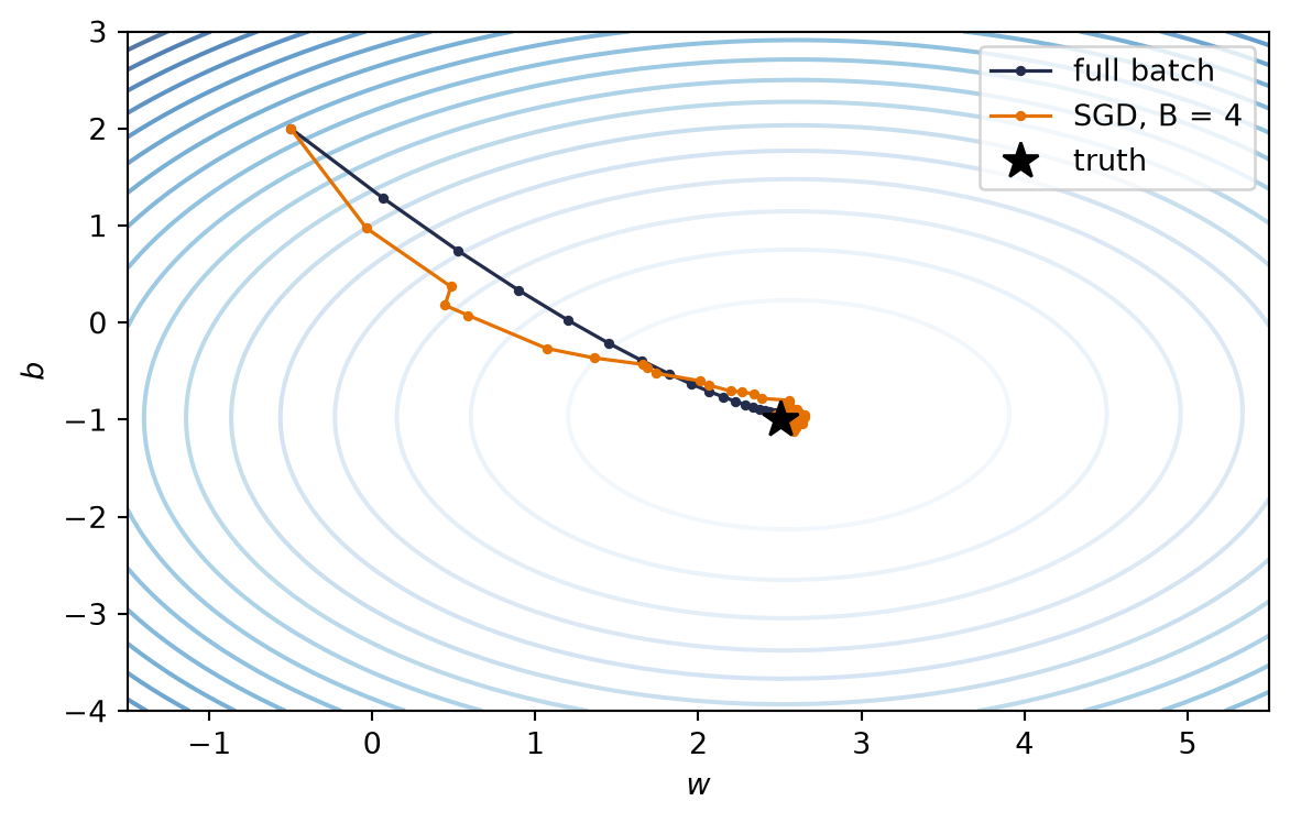
Training with SGD moves through two regimes, a pattern often called semi-convergence: rapid, decisive progress early, then persistent oscillation near the solution. The mechanism is a shifting balance between signal and noise. At any parameter vector, split the minibatch gradient into the full gradient plus a noise vector \(\vect{\xi}_{\mathcal{B}}\) whose mean is zero by the unbiasedness in Equation 4.4:
On our convex least-squares bowl the two regimes are easy to see:
Far from the optimum, signal dominates. The full gradient is large relative to the batch noise, so most batch directions make useful progress, and their mean is the full descent direction.
Near the optimum, noise dominates. The full gradient shrinks toward zero (recall Figure 1.4), but individual batches still disagree (“go left”, “go right”) because different examples pull in different directions. With a fixed learning rate the iterate keeps bouncing inside what we will call the region of confusion:
Generate one least-squares problem and solve for its empirical optimum.
Partition the examples into equal batches and define their gradients.
Compare batch descent directions far from and at the optimum.
Verify that their fixed-point mean equals the full descent direction, then plot both zones.
Figure 4.1: The two zones at fixed parameter vectors. Left: equal-size batch directions vary, but their mean overlaps the full descent direction and points down the convex bowl. Right: at the empirical optimum the full gradient is essentially zero while individual batches still disagree, so finite steps create a region of confusion.
In some regimes the bouncing is not merely tolerable but a feature. A noisy step may perturb the iterate away from a saddle, a narrow basin, or a shallow trap that exact descent would follow more predictably. Minibatch noise can also bias training toward different solutions, and smaller batches sometimes improve generalization. None of these outcomes is guaranteed: the effect depends on the model, data, learning rate, and batch size. For now, treat noise as part of the algorithm, not automatically as a defect or a cure.
Watch the mechanism: why a good batch gradient turns useless
A batch of four instead of all twenty. Is its direction simply a worse one — everywhere?
The chapter's own minibatch update, its unbiasedness statement and its batch_size = 4, on the twenty-point schematic dataset this panel declares: five batches, one iterate, one ruler.
The floor never moved; the signal collapsed. That is why the step must eventually shrink.
0:00 / 0:40
The calculation is readable without playback. Opening this panel loads the optional controls.
The minibatch gradient is unbiased, never a worse gradient; near the optimum the noise does not grow, the signal vanishes, and nothing in this panel is trained.
Scope and caveats
The dataset is schematic: the chapter's eighty points come from torch.manual_seed(6050) and are never printed, so this panel declares twenty of its own — five replicate measurements at each of four x values — on its own line y = −2x + 1.5, which is deliberately not the line Chapter 1's descent panel declares. Every gradient, noise vector, mean, spread, step and ruler reading is computed in the browser from those twenty points. The decomposition, the unbiasedness statement, batch_size = 4 and the two zones are the chapter's.
The region of confusion is about the gradient estimate, not about the loss: it is the exact set where the full gradient is shorter than a typical batch noise vector, and the loss inside it is near its minimum, not confused. Its ellipse is this panel's computed level set; the chapter draws a circle of its own choosing.
The five noise vectors are exactly the same at every (w, b) here because every declared batch carries the same four x values. That rigidity is a property of this declared partition, not a general law: in general a batch's noise varies with the parameters, and only its expectation is pinned to zero.
The arrows are drawn at one declared magnification of the gradient, the same at every time so the shrinking signal is legible; the chapter's figure instead normalises its arrows to unit length in each panel. The step actually taken is the learning rate times the batch gradient — a different, shorter vector that is never drawn.
The batch order is a declared deterministic list: five epochs, each a permutation of the five batches. The chapter prescribes a shuffle, and its own footnote notes that across an epoch, reshuffled batches create path dependence between iterates.
Five batches stand in for the chapter's twenty. More batches would not narrow the spread; a larger batch would, which is a different scene. The remedy for the milling — letting the step size come down — belongs to the next section and is not shown here. Nothing is trained, no loss curve is plotted, and no measured run appears.
Check yourself. Move the iterate to twice its opening displacement from the optimum: (1.8, −1.8) instead of (0.9, −0.9). Does the spread of the five batch directions open wider or close up?
It closes to about half: the widest arrow sits 5.39° off the true direction instead of 10.19°. The five noise vectors never change; doubling the displacement doubles the full gradient, 2.8814 to 5.7628, so the same sideways push bends a direction half as far.
Transcript and keyboard help
Far from the optimum, at (−1.1, 0.6). One wine arrow is the full gradient over all twenty declared points; the ruler under the plane reads its size, 2.8814.
Five batches of four send five thinner arrows from the same point. They spread by at most 10.19 degrees, and every one still points down the bowl.
Each batch arrow is the full one shifted by its own noise vector. The five shifts average to zero, so the dashed outline through the tips is centred exactly on the full arrow's tip; the ruler gains a fixed ink mark at the typical noise size, 0.5561, and the shaded zone below it.
The iterate begins to step, one batch per step, twenty-five steps in five epochs. The full arrow shortens; the outline through the tips keeps its size and shape exactly.
The wine mark on the ruler has slid under the ink one: the full gradient is now smaller than a typical batch noise vector, and the spread has opened past a right angle.
The ellipse where that is true appears round the optimum, the region of confusion. Inside it the five arrows point in five different directions.
The iterate mills inside the ellipse without settling. Its distance from the optimum stays near 0.05 and never falls to zero; the arrows keep disagreeing.
A hollow mark records where the signal started. The full gradient has fallen by a factor of about twenty-two while the ink noise mark has not moved at all. Letting the step size come down is the next section's business, not this panel's.
Silent; paused initially; 1.5× playback. Focus the animation pane: Space or K plays/pauses, arrows seek between beats, Home/End jump, Escape pauses. The scrubber and speed menu also work by keyboard. Reduced-motion mode shows one still per beat; a moving beat rests in the state its caption describes.
4.5 The learning rate
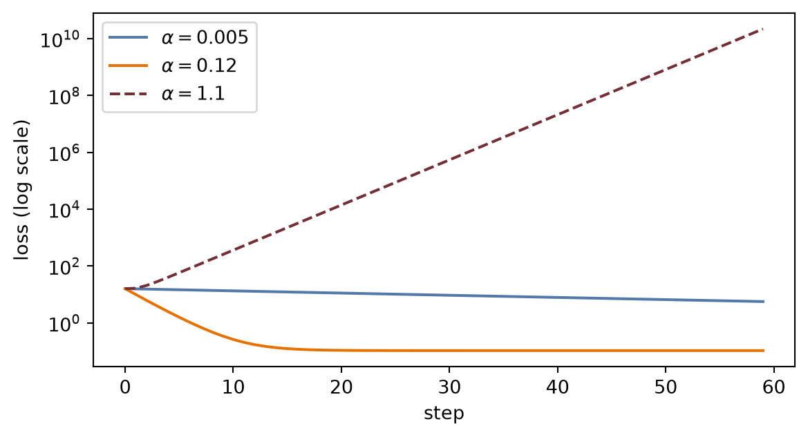
No hyperparameter matters more. The learning rate \(\alpha\) scales every step, and its failure modes are asymmetric: too small wastes your compute budget crawling; too large overshoots the valley and diverges.
Define the reusable losses_for helper.
Open one figure for the three loss curves.
Implement the learning-rate triptych.
Add a legend naming each learning rate and show the figure.
# [1]def losses_for(lr: float, steps: int=60) ->list[float]: w, b, out = torch.tensor(-0.5), torch.tensor(2.0), []for _ inrange(steps): err = (w * x1 + b) - y1 out.append(float((err **2).mean())) w = w - lr *2* (err * x1).mean() b = b - lr *2* err.mean()return out# [2]plt.figure(figsize=(6.2, 3.4))# [3]for lr, style, color in [(0.005, "-", "#5379AA"), (0.12, "-", "#E57200"), (1.1, "--", "#722F37")]: plt.semilogy(losses_for(lr), style, color=color, label=f"$\\alpha = {lr}$")plt.xlabel("step"); plt.ylabel("loss (log scale)")# [4]plt.legend(); plt.tight_layout(); plt.show()
Figure 4.2: Same problem, same steps, three learning rates. Too small crawls; too large overshoots back and forth and climbs; the middle one converges quickly.
TipPractical rule of thumb
For the normalized toy problems here, plain SGD often starts around \(\alpha = 0.1\). That is a scale-calibrated starting point, not a universal constant; Adam, unnormalized features, and very deep models can require very different values. Read the training curves: if the loss crawls, consider raising it; if it oscillates or explodes, lower it. Later in training it often pays to decay the learning rate so the fine-tuning steps get smaller; that is a learning-rate schedule. Warmup starts with a small learning rate and gradually increases it. Recipes for training Transformers (Chapter 16) commonly begin with warmup.
Watch the mechanism: how far one step may go
Three learning rates on one bowl, from one start. Is the largest one simply slower to arrive — or does it never arrive at all?
The chapter's own rates 0.005, 0.12 and 1.1, stepping by its full-batch update rule from its own start w = −0.5, on the one-parameter quadratic bowl this panel declares. Drag α yourself: this bowl has a wall, and it is on that ruler.
Anywhere below the wall it arrives. The chapter starts near 0.1, a tenth of the wall.
0:00 / 0:40
The calculation is readable without playback. Opening this panel loads the optional controls.
A quadratic bowl is the special case that makes a single divergence threshold exist; a real loss surface has no such number, and nothing drawn here is trained.
Scope and caveats
This is full-batch gradient descent on one parameter, not the stochastic version this chapter is about: no minibatch, no noise, no epoch, and no model is fitted. The three rates, the start and the rule of thumb are the chapter's; the bowl is this panel's.
The bowl is declared, not measured: loss (w − 2.5)², curvature 2 — the curvature a standardized feature gives a squared-error loss, which is why the chapter's advice is about normalized toy problems. Its threshold, 2 ÷ 2 = 1, is computed in the browser from the declared curvature; a differently curved bowl has a different one, and the fact that this one lands on 1 is that curvature's coincidence, not a law. The minimum sits at the chapter's generating weight 2.5 and the ball starts at its printed w = −0.5.
Eight steps per rate is this panel's budget; the chapter's own helper runs sixty. The drawn window is w from −4 to 9: at α = 1.1 the ball leaves it after five steps, and from there the picture pins the ball to the frame while the readout keeps the true loss. Landings outside the window are not drawn.
The chapter's figure plots loss against step index on a log axis; this panel deliberately shows the geometry instead, so nothing here is that figure's curve and no step index is an axis. The figure's per-rate colours are not reused: on this picture wine is loss and orange is the parameter.
Decay schedules and warmup are named in the chapter's own rule-of-thumb callout and are out of scope here: α is constant inside every run. The threshold governs this full-batch quadratic only; with minibatch noise a rate well below it can still fail to settle, which is the region of confusion the previous section draws.
Check yourself. Leave the feature unnormalized so the bowl is ten times as curved, c = 20 instead of 2. Which of the chapter's three rates still converges?
Only 0.005. The threshold falls to 2 ÷ 20 = 0.1, so the chapter's middle rate is now past it: its factor is 1 − 0.12 × 20 = −1.4, and the distance to the bottom grows by 1.4 every step. That is what the words normalized toy problems are doing in the rule of thumb.
Transcript and keyboard help
One slope. A ball rests at w = −0.5 on a quadratic bowl whose minimum is at 2.5. The loss there is 9.0000 and the slope is −6.0000, so the dashed arrow spans six units of w — which, on a bowl of curvature 2, is exactly the distance to the point of equal height on the far side.
The first rate, 0.005. The solid arrow is that fraction of the dashed one: 0.0300 of a unit, a hair. Eight steps carry the ball from −0.5 only to −0.2682, and the loss from 9.0000 to 7.6631. Reaching the bottom at this rate takes 568 steps where 0.12 takes 21.
The second rate, 0.12. The same rule and the same eight steps end at w = 2.1661, loss 0.1115. Each step multiplies the distance to the bottom by 0.76.
The third rate, 1.1. The solid arrow is now longer than the dashed one and its tip, at 6.1000, is past the minimum and up the far wall. Predict: does this rate arrive late, or not at all?
The run. Landings at 6.1000, −1.8200, 7.6840 and −3.7208 carry losses 12.9600, 18.6624, 26.8739 and 38.6984 — every one higher than the 9.0000 it started from, and each 1.44 times the one before. The fifth step leaves the picture; after eight the loss is 166.3958.
The wall. The threshold is 2 divided by the curvature, here 2 ÷ 2 = 1. At exactly that rate the step lands on the ring at 5.5, the point of equal height, and the bounce repeats for ever at loss 9.0000.
A tenth under the wall, 0.9. The ball still crosses the valley every step, but each landing is lower: 4.9000, 0.5800, 4.0360 and on down to 1.9967, loss 0.2533.
Back below the wall. The rate glides to 0.12 and the ball rests at the bottom again. The chapter's rule of thumb starts near 0.1, a tenth of this bowl's wall; read the curves, raise a crawling rate and lower an exploding one.
Silent; paused initially; 1.5× playback. Focus the animation pane: Space or K plays/pauses, arrows seek between beats, Home/End jump, Escape pauses. The scrubber and speed menu also work by keyboard. The learning-rate slider has its own arrow keys and never moves the timeline; dragging it pauses playback and draws all eight steps at once, and any timeline action returns to the timeline's own rate. Reduced-motion mode shows one still per beat; a beat that runs rests in the state its caption describes.
4.6 The batch size
The batch size \(B\) sets the operating point on the noise–efficiency trade-off:
Batch size
Character
Trade-off
Small (1–32)
Noisy, exploratory
Sometimes a generalization benefit; slow and less hardware-efficient
Medium (32–256)
Balanced
The usual default; hardware-efficient
Large (256+)
Smooth, high throughput
Less gradient noise; often needs learning-rate and schedule retuning
With independent sampling, gradient standard deviation scales like \(1/\sqrt{B}\): quadrupling the batch roughly halves the jitter. For a uniform subset without replacement, multiply by \(\sqrt{(n-B)/(n-1)}\); when \(B=n\), the noise is exactly zero. For \(B \ll n\) the correction is near one, which is why the simpler rule is useful. There is no universal best setting here, only a dial linking statistics and hardware.
What a batch may estimate, and what it may not
The minibatch argument applies to averages of per-example losses. Other objectives need a separate check.
Case 1: decomposable objectives. When the loss is a mean of per-example terms, \(\loss(\vect{w}) = \E_{x}[\ell(x; \vect{w})]\), a minibatch average is an unbiased estimator of the full objective, and its gradient an unbiased estimator of the full gradient. SGD rests on this unbiasedness, which is why \(B\) is a compute-and-noise dial, not a correctness dial. Cross-entropy, squared error, and every loss in Parts I–III are Case 1, except where BatchNorm in training mode (Chapter 10) makes each example’s term depend on its batch.
Case 2: nonlinear functionals of aggregates. Some quantities are a nonlinear function of an expectation, \(R\bigl(\E_x[s(x)]\bigr)\). A batch plug-in estimate \(R(\bar{s}_B)\) is generally biased (Jensen’s inequality gives the direction when \(R\) is convex or concave), and averaging per-batch values of \(R\) does not converge to the true quantity as training runs longer; only larger batches shrink the bias. Log-of-mean, KL between aggregate distributions, and correlation-style diagnostics belong to this case. For such quantities, either restructure the estimand or declare the bias. The aggregate-posterior trap of Chapter 22 is one example.
Case 3: batch-defined objectives. Sometimes the batch is not estimating anything: it is part of the objective’s definition. A contrastive loss whose denominator ranges over the batch’s own candidates (Chapter 23) is a different objective at \(B=64\) than at \(B=256\): neither is a biased version of the other, and \(B\) becomes part of the protocol, to be reported like any other design choice. Decoding-side analogues exist too: beam width in Chapter 13 defines the search; it does not estimate anything.
A call to .mean() specifies a computation, not its statistical meaning. Depending on how the loss is constructed and the batch is sampled, changing \(B\) can alter the sampling noise, the bias of a plug-in estimate, or the objective itself. Before choosing batch size for speed, write down what the batch calculation estimates or defines, and check the assumptions it requires. Appendix E connects these distinctions to population risk and statistical uncertainty.
Watch the mechanism: what does a bigger batch actually buy?
Four times the batch costs four times as much. Does it buy four times the gradient?
A declared toy least-squares problem with sixty-four examples, evaluated at one fixed parameter vector. Every gradient, the full-batch gradient and the jitter are computed from the numbers this panel declares.
Take the batch to all sixty-four: B equals n, and the noise is exactly zero.
0:00 / 0:40
The calculation is readable without playback. Opening this panel loads the optional controls.
This is sampling noise in the gradient estimate at one fixed parameter vector, not noise in the loss, and nothing here is trained.
Scope and caveats
Both laws are the chapter's; the toy problem is a declared computed variant, so the sixty-four gradients, their average, σ and every jitter reading are computed from the panel's own attributes rather than printed anywhere in the book. The jitter readout and both curves are the exact standard deviation over all uniform subsets of that size; the sixty-four diamonds are sixty-four actual batches from a declared deterministic family — one declared shuffle of the examples, then its sixty-four cyclic windows of length B — so every example sits in exactly B of them and their centre is the full-batch gradient at every B; at B = 1 they are exactly the sixty-four per-example gradients, at B = n they are all the whole population, and in between their spread is close to, not identical with, the curve. This is the chapter's Case 1: the loss is a mean of per-example terms, so a batch average is an unbiased estimate of the full gradient and B is a compute-and-noise dial, not a correctness dial. A batch does not estimate a nonlinear functional of an aggregate without bias, and where the batch defines the objective it is protocol, not an estimator; the chapter separates those cases. Unbiasedness holds at a fixed parameter vector, which is what this scene shows — it is not a claim about successive reshuffled batches along a training run. Cost here is the count of per-example gradients one step needs, not a measured time; larger B costs proportionally more of them, which is the trade the chapter names. The batch size is the scene's one control; dragging it pauses playback, and any timeline action restores the timeline's own value.
Check yourself. A training set of one million examples, batch raised from 100 to 400. By what factor does the gradient's standard deviation change, and how much does the finite-population factor contribute?
Almost exactly one half. One over the square root of four is 0.5; the correction moves only from 0.99995 at B equal to 100 to 0.99980 at 400, so the ratio is 0.49992. For B far below n the correction is near one — the chapter's simpler rule.
Transcript and keyboard help
Sixty-four per-example gradients sit as grey squares in the gradient plane. Their average, the full-batch gradient (7.50, 3.75), is the bold arrow with a ring at its tip.
The jitter scale opens beside the plane. At a batch of one the estimates are the examples themselves, and the standard deviation of the estimate is 11.21.
Held at a batch of one. Quadrupling to four costs four times as much; predict how much of that jitter it removes before releasing.
Released. The batch grows one example at a time to four, and the cloud of sixty-four estimates pulls in toward the true gradient.
At four the jitter is 5.47: the ratio is 0.49, one halving, not the fall to a quarter that proportional thinking expects. Both law curves are drawn.
The batch quadruples again, to sixteen, and the marker slides down the curve toward its flat right-hand end.
At sixteen the jitter is 2.45, a ratio of 0.45. The curve ahead is almost flat: the remaining forty-eight examples have little left to buy.
The batch reaches sixty-four, the whole population. Every one of the sixty-four estimates is the true gradient, the jitter is exactly 0.00, and the dashed independent-sampling law still reads 1.40.
Silent; paused initially; 1.5× playback. Focus the animation pane: Space or K plays/pauses, arrows seek between beats, Home/End jump, Escape pauses. The scrubber, the speed menu and the batch-size slider also work by keyboard; the slider's own keys never move the timeline. Reduced-motion mode holds each beat's state instead of moving between them.
4.7 Momentum: give the ball some mass
Vanilla SGD has one control, \(\alpha\), and in narrow, curved valleys that is not enough: the iterate zigzags across the steep direction while inching along the shallow one. The fix is to give the update a memory. Keep a running velocity that accumulates gradients, and move along the velocity instead of the raw gradient:
with \(\beta \in [0.9, 0.99]\). This is the ball rolling downhill: in directions where gradients keep agreeing, speed builds; in directions where they flip sign every step, they cancel. The zigzag damps itself, and small bumps in the landscape get rolled through rather than obeyed.
The ball analogy can be made precise. A ball of mass \(m\) moving through a viscous fluid with drag coefficient \(\gamma\) over the loss landscape obeys
acceleration comes from the downhill force minus friction. Step it forward with time step \(\Delta t\) and write \(\Delta\vect{w}^{(t)} = \vect{w}^{(t+1)} - \vect{w}^{(t)}\) for the displacement:
This is Equation 4.5 with \(\Delta\vect{w}^{(t)} = -\alpha\,\vect{v}^{(t)}\). So \(\beta\) is the fraction of velocity that survives one step of friction: \(\beta = 0\) is a ball in syrup, which is plain gradient descent, and \(\beta \to 1\) is a frictionless ball that never settles.
Unrolled, the velocity is a geometrically weighted sum of past gradients, \(\vect{v}^{(t)} = \sum_{k \ge 0} \beta^k\,\nabla\loss(\vect{w}^{(t-k)})\), which makes momentum a low-pass filter. A gradient component that keeps its sign is amplified by \(\sum_k \beta^k = 1/(1-\beta)\), ten times at \(\beta = 0.9\); a component that flips sign every step is scaled by \(\sum_k (-\beta)^k = 1/(1+\beta)\), about \(0.53\). The steady downhill signal passes through, while the chatter across the valley and the minibatch noise, which has no preferred sign from step to step, are averaged down relative to it.
Watch the mechanism: how one rule damps a zigzag and speeds a crawl
Momentum gives the update a memory, at the same step length. Does that speed the iterate up in every direction?
The chapter's own velocity recursion and its β ∈ [0.9, 0.99], run at β = 0.9 on the narrow quadratic valley this panel declares: two runs from one start, one step length, and the velocity written out term by term in each direction.
Same rule, same step length: one direction cancelled itself, the other stacked up.
0:00 / 0:40
The calculation is readable without playback. Opening this panel loads the optional controls.
Momentum is not a larger learning rate: both runs here use the same α = 0.05, and a quadratic valley is the easy case that real loss surfaces are not.
Scope and caveats
The valley is schematic: a declared separable quadratic with curvature 40 across and 1 along, started at (0.25, 10) so that both components of the first gradient are exactly 10, and run for eight steps at α = 0.05. The chapter's own ill-conditioned race is seeded and its iterates are never printed, so none of those numbers could be mirrored here. Every gradient, velocity, link and position on this picture is computed in the browser from the declared fixture. The recursion, the range of β and the cancel-or-accumulate behaviour are the chapter's.
β = 0.9 is the low end of the chapter's printed range, and the value its own momentum=0.9 race uses. At that setting the across gradient reverses about every second step rather than literally every step; plain SGD's reverses every single step. The arithmetic is the same either way: a term that disagrees with the accumulated sum subtracts from it.
Plain SGD is the same recursion with nothing kept — β = 0 — so its velocity is the bare gradient, which is what its rail draws; during that sweep the rail reads the gradient at the drawn position, exact at every step and interpolated between. With α = 0.05 and curvature 40, αλ = 2 exactly, so plain SGD's across component sits on the oscillation boundary and neither grows nor dies. A smaller α would damp that zigzag and slow the crawl further, which is the one-dial problem momentum is for.
Drawing devices: the wide layout draws both parameter axes at one scale, 50 pixels per unit, and the narrow layout shows the same window in a taller box, magnifying the across axis about twice; the two gradient legs at the iterate share one declared magnification of 2.2 pixels per gradient unit, so two equal components draw as two equal legs; the two rails share one scale, and the band on each marks ten, the size of the first gradient in both directions. The velocity points uphill, as the recursion writes it, and the step taken is α times it, backwards.
Momentum's along component keeps its sign at every one of the eight steps, and the eighth step carries the iterate 0.6754 past the bottom: speed builds, and a ninth step's gradient would finally point the other way. Nothing is trained, no loss is plotted, and the step counts are not a claim that one optimizer wins at a shared learning rate — the chapter's own race figure is that comparison, and this panel is not it. Nesterov momentum and Adam are named in the chapter and are out of scope here.
Check yourself. Raise β from 0.9 to 0.95 and hold α. One direction's gradient stays at 10 every step; another alternates between +10 and −10. What does each direction's velocity settle to?
The agreeing direction settles at 10/(1−β): 100 at β = 0.9, 200 at β = 0.95 — doubled. The alternating one settles at ±10/(1+β): ±5.2632, then ±5.1282 — slightly smaller. Raising β widens the gap from 19 times to 39 times. More memory does not mean bigger steps everywhere; it sharpens the selection.
Transcript and keyboard help
A narrow valley, drawn as nested level curves of the declared quadratic: steep across, shallow along, with the bottom at the right. One iterate stands at (0.25, 10), and the gradient there splits into two legs of exactly the same length, because both its components are 10.
Plain SGD takes eight steps at α = 0.05. The iterate zigzags across the steep direction — the across gradient flips sign every single step — and inches along the shallow one, ending 6.6342 from the bottom. Its rail carries one link, the current gradient, because plain SGD keeps nothing.
Back to the same start with the same step length, and this time a velocity that remembers, at β = 0.9. Both rails are empty and share one scale; the shaded band on each marks 10, the size of that first gradient. Does the memory speed up both directions?
Two steps, each performed in the order the recursion is written: the running sum shrinks by β, this step's gradient is added to its tip, then the iterate moves. Step one puts 10 on both rails. Step two adds −10 across, which wipes the shrunken 9 down to −1, and +9.5 along, which lifts it to 18.5.
Steps three and four. Two agreeing contributions build the across sum out to −8.9; the reversal at step four wipes it back to 1.79. The along sum, with nothing disagreeing, passes three times one contribution at 30.0162.
Steps five and six. The along sum peaks at 33.7164, more than three contributions, and then eases because its own gradient is dying as the bottom approaches. The across sum keeps folding through zero.
Steps seven and eight. Eight terms on each rail: the across chain has folded back and forth and ends at 2.8355, never once having outgrown the first single contribution of 10; the along chain has marched out to 30.3916.
Both paths together, eight steps each at the same α. Plain SGD is still 6.6342 from the bottom; momentum has arrived and run 0.6754 past it. One rule, one step length, opposite outcomes in the two directions.
Silent; paused initially; 1.5× playback. Focus the animation pane: Space or K plays/pauses, arrows seek between beats, Home/End jump, Escape pauses. The scrubber and speed menu also work by keyboard. Reduced-motion mode shows one still per beat; a moving beat rests in the state its caption describes.
4.8 Adam: adaptive per-parameter steps
Momentum treats every parameter alike, but some parameters sit on steep cliffs while others sit on plains. Adam (adaptive moment estimation) combines three ideas from the same optimization family:2 momentum (accumulate past gradients), per-parameter adaptive learning rates (scale each parameter’s step by its own gradient history), and bias correction (account for both accumulators starting at zero). Formally, Adam applies these elementwise updates:
Because \(\vect{m}^{(0)} = \vect{0}\) and \(\vect{s}^{(0)} = \vect{0}\), dividing by \(1 - \beta_1^t\) and \(1 - \beta_2^t\) corrects the cold-start bias toward zero in early steps; the correction fades away as \(t \to \infty\).
SGD with momentum is lightweight, robust, and often reaches superior generalization when tuned well; Adam provides a versatile default that trains reliably across diverse architectures without intensive tuning.
4.9 The race, on a problem where we know the truth
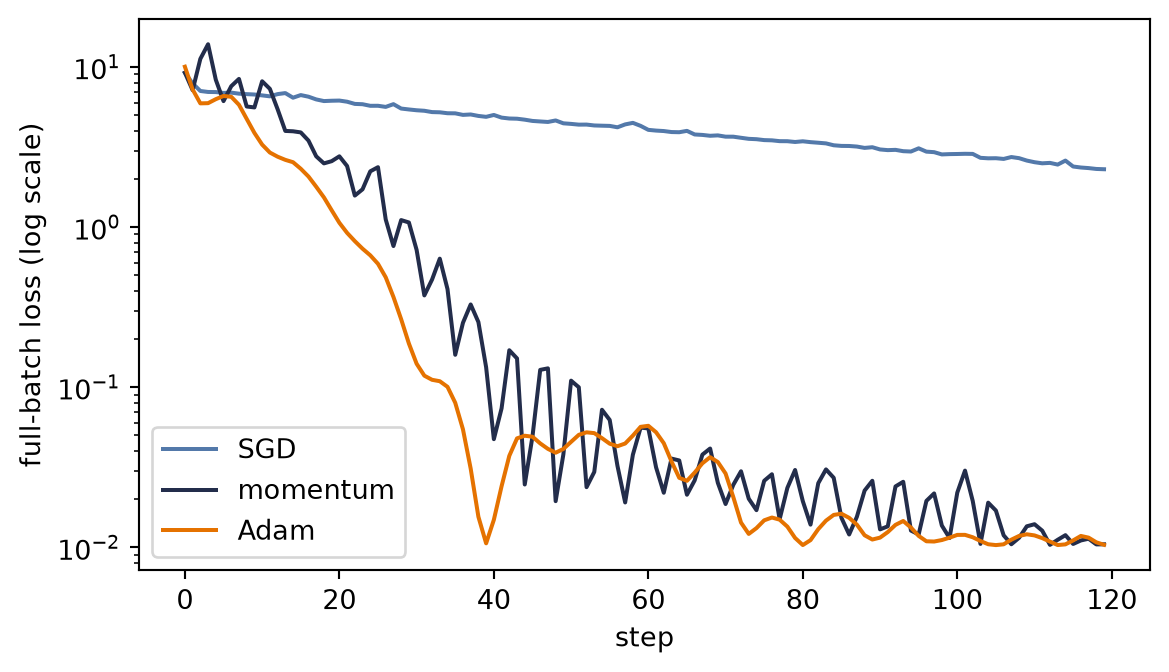
We build a least-squares problem with a deliberately ill-conditioned landscape; the second feature is ten times the scale of the first, so the loss surface is a long narrow valley. We give all three optimizers the same 120-step, 16-example-batch budget, while using learning rates chosen for this toy: \(0.003\) for SGD and momentum, \(0.1\) for Adam. This is a mechanism comparison, not a controlled claim that one optimizer wins at a shared learning rate.
The cell gets the race’s gradients from backward(), as in Chapter 1; Chapter 5 opens that box next.
Fix the seed, draw 256 inputs with feature scales 1 and 10, and form noisy targets from w_true.
Define the reusable race helper.
Implement the optimizer race.
Add a legend naming each optimizer and show the loss curves.
Figure 4.3: The optimizer race on an ill-conditioned valley (feature scales 1 and 10), with an equal step budget and optimizer-appropriate learning rates (\(0.003\) for SGD/momentum, \(0.1\) for Adam). Plain SGD crawls along the shallow direction; momentum damps the zigzag; Adam’s per-parameter scaling largely neutralizes the conditioning.
This is one problem, chosen to expose conditioning; it is not proof that Adam always wins (it does not: plain SGD with momentum, well tuned, still trains many of the best vision models). What the race does show is mechanism: when different directions of the landscape have wildly different steepness, per-direction memory (momentum) and per-parameter scaling (Adam) can reach a loss orders of magnitude below plain SGD’s in the same number of steps. Much of the valley’s narrowness comes from unscaled features. Normalizing the inputs makes the optimizer’s job easier (Exercise 5).
4.10 Regularization during training
Weight decay, dropout, and early stopping regularize training in different ways. Weight decay modifies parameter updates, dropout randomly masks activations, and early stopping uses validation performance to determine training duration.
Weight decay
Under plain SGD, adding an \(L_2\) penalty \(\frac{\lambda}{2}\|\vect{w}\|_2^2\) to the loss gives
The penalty introduces a shrinkage term, connecting weight decay to the ridge regression of Chapter 1.
Many PyTorch optimizers expose a weight_decay argument, but its implementation matters. Under Adam, an \(L_2\) penalty contributes \(\lambda\vect{w}\) to the gradient. This contribution is processed through the moment estimates and the coordinate-wise scaling of Equation 4.6, so it does not produce the same uniform shrinkage. AdamW applies \(\vect{w} \leftarrow (1-\alpha\lambda)\vect{w}\) separately from the adaptive gradient update. Training recipes often exclude bias and normalization parameters from this decay.
Dropout
Dropout randomly sets activations to zero during training. Let \(h_i\) be one hidden activation, \(p\) its drop probability, and \(q=1-p\) the probability that it is retained. With inverted dropout, an independent mask \(r_i\sim\operatorname{Bernoulli}(q)\) gives
At evaluation time, dropout is disabled and the activation remains \(h_i\), with no rescaling. PyTorch’s nn.Dropout(p) uses this convention: model.train() enables its masking, and model.eval() disables it. The choice changes the computation, not just its execution speed.
Here is the mechanism written directly, followed by a small seeded check. The empirical training mean is close to the input, while evaluation is deterministic and leaves the input unchanged:
Define the reusable inverted_dropout helper.
Fix the seed and average 20,000 inverted_dropout draws of the four-entry h at p = 0.25.
Implement inverted dropout and verify its scale.
# [1]def inverted_dropout( h: torch.Tensor, p: float, training: bool=True) -> torch.Tensor:ifnot training:return hifnot0.0<= p <1.0:raiseValueError("p must satisfy 0 <= p < 1") q =1.0- p mask = (torch.rand_like(h) < q).to(h.dtype)return mask * h / q# [2]torch.manual_seed(6050)h = torch.tensor([1.0, -2.0, 4.0, 0.5])draws = torch.stack([inverted_dropout(h, p=0.25) for _ inrange(20_000)])mean_output = draws.mean(0)# [3]print("training mean:", [round(v, 4) for v in mean_output.tolist()])print(f"max |mean - h|: {(mean_output - h).abs().max():.4f}")print("evaluation:", inverted_dropout(h, p=0.25, training=False).tolist())
training mean: [1.0025, -2.0057, 4.0064, 0.5024]
max |mean - h|: 0.0064
evaluation: [1.0, -2.0, 4.0, 0.5]
Dropout also has an approximate ensemble interpretation. Training uses many masked subnetworks with shared weights, while evaluation uses the full network. Preserving the conditional mean of each masked activation does not make the full network’s prediction equal to the average prediction of those subnetworks. Nonlinear transformations generally do not commute with expectation:
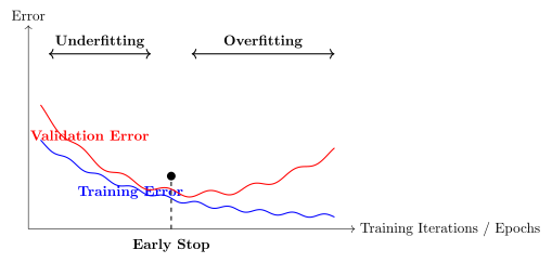
Monitor validation loss during training. Early stopping limits training when validation performance stops improving, even if training loss continues to decrease. Retain the checkpoint with the lowest validation loss. Figure 4.4 illustrates this choice along one training trajectory.
Figure 4.4: Early stopping as model selection along one training trajectory. In this schematic, validation loss eventually increases while training loss continues to decrease. The checkpoint at the validation minimum is retained.
NoteCheck yourself
Write one parameter update, then answer the following questions.
Under what sampling assumptions is a minibatch gradient unbiased, and why does it vary between batches?
What information from earlier gradients is used by momentum and Adam?
Why is an \(L_2\) penalty under Adam different from uniform weight decay, and what does AdamW change?
Why does inverted dropout need no rescaling at evaluation time, and how does leaving dropout active change validation predictions?
4.11 Okay, so: the training loop
The pieces above fit into one training loop:
Instantiate the parameters \(\vect{w}^{(0)}\): PyTorch layers initialize their weights automatically when they are created (Chapter 5 analyzes why that initial scale governs trainability).
For each epoch: shuffle, split into minibatches of size \(B\).
For each batch: training-mode forward pass (including dropout, if used) \(\rightarrow\) loss (your noise model in disguise) \(\rightarrow\) backward pass for the gradients \(\rightarrow\) optimizer step (\(\alpha\), momentum or Adam, weight decay).
Switch to evaluation mode for validation; watch the curve, schedule the learning rate, and stop early when it turns.
Here is that recipe as a tested function, Listing 4.1. Later chapters import it and show only their model builder and their budget:
Declare one reusable interface for the model factory, data, and training budget.
Seed before constructing the model and optimizer.
Reshuffle the examples and visit every minibatch each epoch.
Predict, measure cross-entropy, backpropagate, and update.
Return the trained model as the experiment artifact.
"""Listing 4.1 — the supervised training loop, importable.Chapter 4 derives this loop and prints it; Chapters 6 and 9 import it andprint only their deltas (the model builder and the budget). The loop is thebook's canonical minibatch recipe: seed, build, then repeatpredict -> measure -> step over reshuffled minibatches."""from collections.abc import Callableimport torchimport torch.nn.functional as Ffrom torch import nn# [1]def fit_supervised( model_fn: Callable[[], nn.Module], X: torch.Tensor, y: torch.Tensor,*, epochs: int, batch: int=64, lr: float=1e-3, seed: int=6050,) -> nn.Module:"""Train a fresh model on (X, y) with cross-entropy and Adam. Seeding precedes construction, so a given (model_fn, seed) pair always starts from the same tensors; each epoch reshuffles example order. """# [2] torch.manual_seed(seed) model = model_fn() opt = torch.optim.Adam(model.parameters(), lr=lr)# [3]for _ inrange(epochs): perm = torch.randperm(len(X))for i inrange(0, len(X), batch): idx = perm[i : i + batch]# [4] loss = F.cross_entropy(model(X[idx]), y[idx]) opt.zero_grad() loss.backward() opt.step()# [5]return model
Two reading notes. Seeding precedes construction, so one (model_fn, seed) pair always trains from the same starting tensors, which a paired comparison requires. And the loss line is a Case 1 estimator: a per-example objective averaged over a shuffled minibatch is an unbiased estimate of the full-data loss, which is why the minibatch size is a compute-and-noise dial, not a correctness dial (Section 4.6.1).
One step in that loop is still a black box: the backward pass for the gradients. Computing millions of partial derivatives for about twice the arithmetic of one forward pass is the subject of Chapter 5.
Sources and further reading
Tieleman and Hinton, “Lecture 6.5 — RMSProp,” COURSERA: Neural Networks for Machine Learning (2012): the original public provenance for RMSProp’s running average of squared gradients.
Gilbert Strang, Linear Algebra and Learning from Data, §VI.4–VI.5, is a classical numerical-linear-algebra treatment: gradient descent, condition numbers, and momentum on quadratic bowls (§VI.4), and stochastic gradient descent’s semi-convergence, unbiased-gradient assumption, and convergence in expectation (§VI.5, especially pp. 361–365).
(Pencil.) Prove Equation 4.4 for sampling with replacement: if \(i\) is drawn uniformly from \(\{1,\dots,n\}\), show \(\E[\nabla \ell_i(\vect{w})] = \frac{1}{n}\sum_j \nabla \ell_j(\vect{w})\). Where exactly does the argument use uniformity?
(Code.) On the two-zones problem, run 100 SGD steps from the far point \((-0.5, 2)\) with one fixed learning rate (for example \(\alpha = 0.05\)), drawing each batch without replacement from the 80 examples, for \(B \in \{1, 4, 16, 80\}\). Measure the radius of the region of confusion as the root-mean-square distance of the last 30 iterates from the optimum, \(\bigl(\tfrac{1}{30}\sum_{t=71}^{100}\lVert\vect{w}^{(t)}-\vect{w}^\star\rVert_2^2\bigr)^{1/2}\). How does it scale with \(B\)? Compare against \(1/\sqrt{B}\) first, then include the finite-population correction \(\sqrt{(n-B)/(n-1)}\). Why must the noise vanish at \(B=80\)?
(Code.) Add a learning-rate schedule to the race: halve \(\alpha\) every 30 steps for plain SGD. How much of the gap to momentum does scheduling close? What does that tell you about what momentum is really fixing here?
(Code.) Sweep momentum’s \(\beta \in \{0, 0.5, 0.9, 0.99\}\) in the race. Explain the failure mode at the top end using the ball analogy.
(Code.) Rescale each column of Xr to unit standard deviation and rerun all three optimizers. The columns are already zero-mean and the model has no intercept, so this scaling is full standardization here. Retune SGD’s learning rate, which was sized for the old steep direction, and compare full-batch losses rather than weights, since rescaling changes the parameterization. How much of Adam’s advantage evaporates? State the practical moral in one sentence.
(Pencil.) (a) From Equation 4.7, show that \(\operatorname{Var}(\widetilde{h}_i\mid h_i)=p h_i^2/(1-p)\). (Code.) (b) Estimate that variance for \(p\in\{0.1,0.5,0.9\}\) using the seeded check. What happens to signal noise as \(p \to 1\), and what defect does leaving masking on introduce at evaluation? (Think about determinism and variance, not the mean, which inverted dropout already preserves.)
At a fixed \(\vect{w}\), a subset of size \(B\) drawn without replacement is unbiased, and its variance is the with-replacement variance times the finite-population correction \((n-B)/(n-1)\), which reaches zero at \(B=n\). Across an epoch, however, reshuffled batches create path dependence between iterates; dedicated random-reshuffling theory handles that sequence.↩︎
The per-parameter denominator is RMSProp. Adam adds bias-corrected first moments and names RMSProp directly.↩︎