Deep Learning: Making It Learnable

Heman Shakeri

Appendix A — Linear Algebra and the SVD

You have used linear algebra since the first page of this book. A dot product scored a pattern in Chapter 1. Matrix products routed queries to keys in Chapter 13. Low-rank factors limited an update in Chapter 17, and PCA supplied the flat reconstruction baseline in the autoencoder interlude. Why return to the subject now?

Because the notation is compact enough to hide mistakes—a product can be legal while representing the wrong convention; an inverse can exist while being the wrong computation; and an SVD can be exact while its singular vectors are not uniquely identifiable. This appendix gathers the geometry and the PyTorch habits that let you audit those cases. It is a working reference—not a compressed linear-algebra course.

A.1 Read the map from its dimensions

Let us start with one concrete map. A matrix \(\matr{A}\in\mathbb{R}^{m\times n}\) accepts a column vector \(\vect{x}\in\mathbb{R}^{n}\) and returns \(\vect{y}=\matr{A}\vect{x}\in\mathbb{R}^{m}\). The input has \(n\) coordinates, the output has \(m\), and column \(j\) of \(\matr{A}\) records where the \(j\)th standard basis vector goes. Once those columns are known, every input follows—by linear combination:

\[ \matr{A}\vect{x} =x_1\matr{A}_{:1}+\cdots+x_n\matr{A}_{:n}. \]

That is the geometric reading of matrix multiplication. The computational reading is the same operation viewed by rows: output coordinate \(i\) is the dot product \(\matr{A}_{i:}\vect{x}\). Switching between the two views is useful—the columns show what the map can produce, while the rows show how each output is measured.

A map \(T\) is linear when, for every pair of vectors and scalars,

\[ T(a\vect{x}+b\vect{z})=aT(\vect{x})+bT(\vect{z}). \]

This definition includes \(T(\vect{0})=\vect{0}\)—a fact worth checking before calling an operation linear. Adding a nonzero bias breaks that condition, so \(\vect{x}\mapsto\matr{A}\vect{x}+\vect{b}\) is affine. PyTorch’s nn.Linear uses that affine form by default despite its name—a useful vocabulary distinction whenever a theorem assumes a genuinely linear map.

One vector on paper, a row batch in PyTorch

The mathematical convention above stores one sample as a column. The book’s PyTorch code stores \(B\) samples as rows of \(\matr{X}\in\mathbb{R}^{B\times n}\). The same map is therefore

\[ \matr{Y}=\matr{X}\matr{A}^{\top} \in\mathbb{R}^{B\times m}. \tag{A.1}\]

PyTorch stores an nn.Linear(n, m) weight with shape \((m,n)\), and its matrix part uses exactly this row-batch convention. With the default bias, the full affine operation is \(\matr{Y}=\matr{X}\matr{A}^{\top}+\vect{1}\vect{b}^{\top}\). What do we expect before running the code? One contract is already fixed—the batch shaped \((3,2)\) multiplied by \(\matr{A}^{\top}\in\mathbb{R}^{2\times2}\) must remain \((3,2)\). Let us check the values as well as the shapes.

Code: reconcile column-vector algebra with PyTorch row batches

import math

import matplotlib.pyplot as plt
import torch

torch.set_default_dtype(torch.float64)
torch.manual_seed(6050)

transform = torch.tensor([[2.0, 1.0], [-1.0, 3.0]])       # (out, in)
vector = torch.tensor([4.0, 2.0])                         # (in,)
batch = torch.tensor([[1.0, 0.0], [2.0, 1.0], [0.0, -1.0]])  # (B, in)

row_outputs = batch @ transform.T                         # (B, out)
column_outputs = (transform @ batch.T).T

rotation = torch.tensor([[0.0, -1.0], [1.0, 0.0]])
scaling = torch.tensor([[2.0, 0.0], [0.0, 3.0]])
order_probe = torch.tensor([1.0, 2.0])
rotate_then_scale = (scaling @ rotation) @ order_probe
scale_then_rotate = (rotation @ scaling) @ order_probe

assert torch.equal(transform @ vector, torch.tensor([10.0, 2.0]))
assert torch.equal(row_outputs, column_outputs)
assert not torch.equal(rotate_then_scale, scale_then_rotate)

print("single output:", (transform @ vector).tolist())
print("row batch shapes:", tuple(batch.shape), "->", tuple(row_outputs.shape))
print("row batch outputs:", row_outputs.tolist())
print("rotate then scale:", rotate_then_scale.tolist())
print("scale then rotate:", scale_then_rotate.tolist())

single output: [10.0, 2.0]
row batch shapes: (3, 2) -> (3, 2)
row batch outputs: [[2.0, -1.0], [5.0, 1.0], [-1.0, -3.0]]
rotate then scale: [-4.0, 3.0]
scale then rotate: [-6.0, 2.0]

The two batch calculations agree exactly. The composition check exposes a second habit: matrix order reads from right to left. If \(\matr{R}\) rotates and \(\matr{S}\) scales, then \(\matr{S}\matr{R}\vect{x}\) rotates first. Reversing the factors changes the answer from \((-4,3)\) to \((-6,2)\)—both products are dimensionally legal, so a shape check alone cannot catch the semantic mistake.

A three-line shape audit

Before every product, write the operand shapes; identify which two dimensions contract; then write the surviving shape. For high-rank tensors, @ treats the last two axes as matrix axes and the leading axes as batch axes. Broadcasting and physical layout are gathered in Appendix B.

A.2 Span, rank, and orthogonality

The span of a set of vectors is every linear combination they can produce. A basis spans a space without redundant directions. These words make a matrix’s geometry precise:

The column space \(\operatorname{col}(\matr{A})\subseteq\mathbb{R}^{m}\) is every reachable output \(\matr{A}\vect{x}\).
The null space \(\operatorname{null}(\matr{A})\subseteq\mathbb{R}^{n}\) is every input direction that the map sends to zero.
The rank is the dimension of the column space—the number of independent output directions. It is at most \(\min(m,n)\), and it counts independent input directions that survive the map.

The dot product adds geometry. For \(\vect{x},\vect{z}\in\mathbb{R}^{n}\),

\[ \vect{x}^{\top}\vect{z} =\norm{\vect{x}}_2\norm{\vect{z}}_2\cos\theta. \]

It is zero when nonzero vectors are perpendicular. If \(\matr{Q}\in\mathbb{R}^{m\times k}\) has orthonormal columns, so that \(\matr{Q}^{\top}\matr{Q}=\matr{I}_k\), then

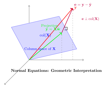
\[ \matr{P}=\matr{Q}\matr{Q}^{\top}, \qquad \widehat{\vect{y}}=\matr{P}\vect{y} \tag{A.2}\]

projects \(\vect{y}\) onto \(\operatorname{col}(\matr{Q})\). The projector is symmetric and idempotent: \(\matr{P}^{\top}=\matr{P}\) and \(\matr{P}^2=\matr{P}\). The residual \(\vect{r}=\vect{y}-\widehat{\vect{y}}\) is orthogonal to every column of \(\matr{Q}\).

This is the picture behind the normal equations in Chapter 1—the fit uses every reachable direction and leaves an orthogonal residual. It also explains why the autoencoder interlude compares PCA and a tied linear autoencoder through their projectors, not through individual basis vectors. Rotating or reflecting an orthonormal basis changes its coordinates while leaving \(\matr{Q}\matr{Q}^{\top}\) unchanged—the subspace is the stable object.

Geometric projection of y onto the column space of X, with residual e drawn perpendicular to the fitted vector. — Figure A.1: Projection separates what the columns can express from what they cannot. The fitted vector \(\widehat{\vect{y}}\) lies in the column space; the residual is orthogonal to every column direction. The diagram labels that residual \(\vect{e}=\vect{y}-\widehat{\vect{y}}\); the appendix uses \(\vect{r}\) for the same quantity.

A.3 Solve the problem you actually have

Suppose \(\matr{A}\in\mathbb{R}^{n\times n}\) is nonsingular and \(\vect{b}\in\mathbb{R}^{n}\). The equation \(\matr{A}\vect{x}=\vect{b}\) has one solution. The notation \(\vect{x}=\matr{A}^{-1}\vect{b}\) describes it, but it does not prescribe a good algorithm. In PyTorch, use torch.linalg.solve(A, b)—it solves the system without first materializing an inverse.

Most data problems are rectangular—the target may not lie in the column space. For \(\matr{X}\in\mathbb{R}^{N\times d}\) and \(\vect{y}\in\mathbb{R}^{N}\), least squares asks for

\[ \widehat{\vect{w}} =\argmin_{\vect{w}\in\mathbb{R}^{d}} \norm{\matr{X}\vect{w}-\vect{y}}_2^2. \tag{A.3}\]

At an optimum, the residual—a record of what the columns cannot explain— \(\vect{r}=\vect{y}-\matr{X}\widehat{\vect{w}}\) satisfies \(\matr{X}^{\top}\vect{r}=\vect{0}\). If \(\matr{X}\) has full column rank, expanding that condition gives the familiar normal-equation expression

\[ \widehat{\vect{w}} =(\matr{X}^{\top}\matr{X})^{-1}\matr{X}^{\top}\vect{y}. \]

Again, this is an identity—not the preferred recipe. torch.linalg.lstsq(X, y) works on the rectangular system directly. It also reports rank-related information for supported algorithms, which matters when columns are redundant or nearly so.

Why avoid forming \(\matr{X}^{\top}\matr{X}\)? Let the nonzero singular values of a full-column-rank matrix be \(\sigma_{\max}\) and \(\sigma_{\min}\). Its 2-norm condition number is

\[ \kappa_2(\matr{X}) =\frac{\sigma_{\max}}{\sigma_{\min}}, \qquad \kappa_2(\matr{X}^{\top}\matr{X}) =\kappa_2(\matr{X})^2. \tag{A.4}\]

Directions that were difficult to distinguish become much more difficult after the square—the next cell uses a matrix whose columns differ by only \(0.001\).

Code: solve square and rectangular systems, then expose conditioning

square = torch.tensor([[3.0, 1.0], [1.0, 2.0]])
right_hand_side = torch.tensor([9.0, 8.0])
solution = torch.linalg.solve(square, right_hand_side)

design = torch.tensor([[1.0, 0.0], [1.0, 1.0],
                       [1.0, 2.0], [1.0, 3.0]])           # (N, d)
target = torch.tensor([1.0, 2.0, 2.0, 4.0])              # (N,)
least_squares = torch.linalg.lstsq(design, target)
weights = least_squares.solution
residual = target - design @ weights
normal_residual = torch.linalg.vector_norm(design.T @ residual)

near_collinear = torch.tensor([[1.0, 1.0], [1.0, 1.001]])
condition = torch.linalg.cond(near_collinear)
normal_condition = torch.linalg.cond(near_collinear.T @ near_collinear)

assert torch.allclose(solution, torch.tensor([2.0, 3.0]))
assert normal_residual < 1e-12
assert torch.allclose(normal_condition, condition.square(), rtol=1e-7)

print(f"solve solution: ({solution[0]:.6f}, {solution[1]:.6f})")
print(f"least-squares solution: ({weights[0]:.6f}, {weights[1]:.6f})")
print(f"normal-equation residual: {normal_residual:.3e}")
print(f"condition(A): {condition:.6f}")
print(f"condition(A.T @ A): {normal_condition:.6f}")
print(f"squaring ratio: {normal_condition / condition.square():.12f}")

solve solution: (2.000000, 3.000000)
least-squares solution: (0.900000, 0.900000)
normal-equation residual: 2.220e-15
condition(A): 4002.000750
condition(A.T @ A): 16016009.992981
squaring ratio: 0.999999999312

The least-squares solution is \((0.9,0.9)\), and the norm of \(\matr{X}^{\top}\vect{r}\) is about \(2.2\times10^{-15}\) in float64. For the nearly collinear matrix, the condition number grows from about \(4.002\times10^3\) to \(1.602\times10^7\) after forming \(\matr{A}^{\top}\matr{A}\)—the predicted square to displayed precision.

More digits do not repair missing information

Float64 makes this tiny audit easier to inspect; it does not make an ill-conditioned problem well-conditioned. Check inputs with torch.isfinite, inspect torch.linalg.cond or the singular values when stability matters, and verify the residual. Near a numerical-rank threshold, reported rank and solutions can change with dtype, tolerance, algorithm, or platform. Appendix C separates those numerical questions from the underlying algebra.

A.4 Eigenvectors are a square-matrix special case

An eigenvector asks whether one nonzero direction stays on its own line under a square map:

\[ \matr{A}\vect{v}=\lambda\vect{v}, \qquad \matr{A}\in\mathbb{R}^{n\times n}. \]

This question requires the input and output spaces to be the same—even then, a real matrix may have complex eigenvalues or too few independent eigenvectors. Symmetric real matrices are the friendly case: their eigenvalues are real and they admit an orthonormal eigenbasis. Use torch.linalg.eigh, rather than the more general eig, when that symmetry is known.

Deep-learning weight matrices are often rectangular, so we need a decomposition that uses one set of directions in the input space and another in the output space. That is the role of the singular value decomposition—the two spaces no longer need to be the same.

A.5 SVD: two spaces and one ordered scale

Let \(\matr{A}\in\mathbb{R}^{m\times n}\) and set \(k=\min(m,n)\). Its reduced SVD is

\[ \matr{A}=\matr{U}\matr{\Sigma}\matr{V}^{\top}, \tag{A.5}\]

with

\[ \matr{U}\in\mathbb{R}^{m\times k},\qquad \matr{\Sigma}=\operatorname{diag}(\sigma_1,\ldots,\sigma_k) \in\mathbb{R}^{k\times k},\qquad \matr{V}^{\top}\in\mathbb{R}^{k\times n}. \]

The singular values are real, nonnegative, and ordered—a scale ledger from the most amplified direction to the least: \(\sigma_1\geq\cdots\geq\sigma_k\geq0\). The columns satisfy

\[ \matr{A}\vect{v}_i=\sigma_i\vect{u}_i, \qquad \matr{A}^{\top}\vect{u}_i=\sigma_i\vect{v}_i \quad\text{when }\sigma_i>0. \tag{A.6}\]

Geometrically, \(\matr{V}^{\top}\) selects orthogonal input coordinates, \(\matr{\Sigma}\) scales or removes them, and \(\matr{U}\) places the result in the output space. Strang’s rotate–stretch–rotate picture is useful in the square, two-dimensional case—but orthogonal factors may include reflections. In a reduced rectangular SVD, \(\matr{V}^{\top}\) maps \(n\) coordinates to \(k\) and \(\matr{U}\) maps those \(k\) coordinates into an \(m\)-dimensional output; the dimension change belongs to the whole factorization, not to the displayed \(k\times k\) diagonal matrix alone.

The eigenvalue bridge follows—without using \(\matr{A}^{\top}\matr{A}\) as a numerical SVD algorithm:

\[ \matr{A}^{\top}\matr{A}\vect{v}_i =\sigma_i^2\vect{v}_i, \qquad \matr{A}\matr{A}^{\top}\vect{u}_i =\sigma_i^2\vect{u}_i. \tag{A.7}\]

torch.linalg.svd(A, full_matrices=False) returns U, S, Vh; S is a one-dimensional tensor, not a diagonal matrix. Scaling the columns of U reconstructs the map without building that diagonal matrix: (U * S.unsqueeze(-2)) @ Vh.

Rank-one layers and truncation

Expanding Equation A.5 gives

\[ \matr{A}=\sum_{i=1}^{k}\sigma_i\vect{u}_i\vect{v}_i^{\top}. \tag{A.8}\]

Each outer product has rank at most one—a complicated map becomes an ordered sum of simple layers. Keeping the first \(r\) terms gives

\[ \matr{A}_r =\sum_{i=1}^{r}\sigma_i\vect{u}_i\vect{v}_i^{\top}. \tag{A.9}\]

For \(0\leq r<k\), the Eckart–Young–Mirsky result makes “best” precise—among matrices of rank at most \(r\), \(\matr{A}_r\) minimizes both the operator-norm and Frobenius-norm errors, with

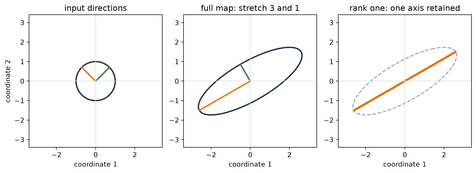
\[ \norm{\matr{A}-\matr{A}_r}_2=\sigma_{r+1}, \qquad \norm{\matr{A}-\matr{A}_r}_F^2 =\sum_{i=r+1}^{k}\sigma_i^2. \tag{A.10}\]

Let us construct a map whose singular values are exactly 3 and 1. The full map sends the unit circle to an ellipse. The rank-one approximation keeps the longer axis and collapses the other—a visible instance of the theorem rather than a claim inferred from a complicated dataset.

Figure code: decompose a known map and expose the rank-one error

left_angle, right_angle = math.pi / 6.0, -math.pi / 4.0
left_basis = torch.tensor([
    [math.cos(left_angle), -math.sin(left_angle)],
    [math.sin(left_angle), math.cos(left_angle)],
])
right_basis = torch.tensor([
    [math.cos(right_angle), -math.sin(right_angle)],
    [math.sin(right_angle), math.cos(right_angle)],
])
linear_map = left_basis @ torch.diag(torch.tensor([3.0, 1.0])) @ right_basis.T

u, singular_values, vh = torch.linalg.svd(linear_map, full_matrices=False)
reconstructed = (u * singular_values.unsqueeze(0)) @ vh
rank_one = (u[:, :1] * singular_values[:1]) @ vh[:1]
frobenius_error = torch.linalg.matrix_norm(linear_map - rank_one, ord="fro")
operator_error = torch.linalg.matrix_norm(linear_map - rank_one, ord=2)
eigenvalues = torch.linalg.eigvalsh(linear_map.T @ linear_map)

assert torch.allclose(singular_values, torch.tensor([3.0, 1.0]))
assert torch.allclose(linear_map, reconstructed)
assert torch.allclose(eigenvalues.flip(0), singular_values.square())
assert torch.allclose(frobenius_error, singular_values[1:].square().sum().sqrt())
assert torch.allclose(operator_error, singular_values[1])

print("singular values:", [round(value, 6) for value in singular_values.tolist()])
print(f"reconstruction max error: {(linear_map - reconstructed).abs().max():.3e}")
print("eigenvalues of A.T @ A:", [round(value, 6) for value in eigenvalues.tolist()])
print(f"rank-one Frobenius error: {frobenius_error:.6f}")
print(f"rank-one operator error: {operator_error:.6f}")

angles = torch.linspace(0.0, 2.0 * math.pi, 361)
unit_circle = torch.stack((torch.cos(angles), torch.sin(angles)))  # (2, points)
full_image = linear_map @ unit_circle
rank_one_image = rank_one @ unit_circle

fig, axes = plt.subplots(1, 3, figsize=(10, 3.4))
axes[0].plot(unit_circle[0], unit_circle[1], color="#232D4B", lw=2)
for index, color in enumerate(["#E57200", "#2E7D32"]):
    direction = vh[index]
    axes[0].plot([0.0, direction[0]], [0.0, direction[1]], color=color, lw=2)
axes[0].set_title("input directions")

axes[1].plot(full_image[0], full_image[1], color="#232D4B", lw=2)
for index, color in enumerate(["#E57200", "#2E7D32"]):
    scaled_axis = singular_values[index] * u[:, index]
    axes[1].plot([0.0, scaled_axis[0]], [0.0, scaled_axis[1]], color=color, lw=2)
axes[1].set_title("full map: stretch 3 and 1")

axes[2].plot(full_image[0], full_image[1], color="#9AA5B1", lw=1.5, ls="--")
axes[2].plot(rank_one_image[0], rank_one_image[1], color="#E57200", lw=3)
axes[2].set_title("rank one: one axis retained")

for axis in axes:
    axis.axhline(0.0, color="#D6DCE5", lw=0.8)
    axis.axvline(0.0, color="#D6DCE5", lw=0.8)
    axis.set_aspect("equal")
    axis.set_xlim(-3.4, 3.4)
    axis.set_ylim(-3.4, 3.4)
    axis.set_xlabel("coordinate 1")
axes[0].set_ylabel("coordinate 2")
plt.tight_layout()
plt.show()

singular values: [3.0, 1.0]
reconstruction max error: 8.882e-16
eigenvalues of A.T @ A: [1.0, 9.0]
rank-one Frobenius error: 1.000000
rank-one operator error: 1.000000

Three panels show a unit circle with two orthogonal input directions, its elliptical image with axes of lengths three and one, and the rank-one image as a line segment over a dashed ellipse. — Figure A.2: A two-dimensional SVD with singular values 3 and 1. The right singular vectors choose orthogonal input directions; the left singular vectors orient the ellipse’s scaled axes. Keeping one rank-one term collapses the ellipse to its longer axis. Because there is only one omitted singular value, both the operator error and Frobenius error are exactly 1.

The singular values are unique, but their vectors need not be—each singular pair can flip sign without changing \(\matr{A}\). When singular values repeat, any orthonormal basis of the repeated subspace is valid. Accordingly, tests should compare the reconstruction or a subspace projector—not demand one particular U or Vh.

Magnitude is not meaning

A truncated SVD is optimal for the matrix norms in Equation A.10. That does not prove that a large singular direction is semantic signal or that a small one is noise. Feature scaling, the downstream task, and the data-generating process decide whether discarding a direction is useful. A low-rank weight approximation can be close as a matrix yet still change a model’s predictions; measure the downstream behavior.

A.6 Batched linear algebra

The same decomposition can be applied to many matrices at once—the last two dimensions remain the matrix. For an input shaped \((B,m,n)\), torch.linalg.svd(..., full_matrices=False) returns shapes \((B,m,k)\), \((B,k)\), and \((B,k,n)\). The singular values need one inserted axis so they scale columns of U rather than a batch axis.

Code: reconstruct a batch of rectangular matrices from reduced SVDs

rectangular_batch = torch.stack((
    torch.tensor([[3.0, 0.0], [0.0, 1.0], [0.0, 0.0]]),
    torch.tensor([[0.0, 2.0], [0.5, 0.0], [0.0, 0.0]]),
))                                                          # (B, m, n)

batch_u, batch_s, batch_vh = torch.linalg.svd(
    rectangular_batch, full_matrices=False
)
batch_reconstruction = (batch_u * batch_s.unsqueeze(-2)) @ batch_vh

assert torch.allclose(rectangular_batch, batch_reconstruction)

print("A batch:", tuple(rectangular_batch.shape))
print("U, S, Vh:", tuple(batch_u.shape), tuple(batch_s.shape), tuple(batch_vh.shape))
print(
    f"batched reconstruction max error: "
    f"{(rectangular_batch - batch_reconstruction).abs().max():.3e}"
)
print("singular values by matrix:", batch_s.tolist())

A batch: (2, 3, 2)
U, S, Vh: (2, 3, 2) (2, 2) (2, 2, 2)
batched reconstruction max error: 0.000e+00
singular values by matrix: [[3.0, 1.0], [2.0, 0.5]]

The leading dimension stays a batch throughout. A Python loop and a batched call are mathematically equivalent here, but floating-point implementations need not be bitwise identical. Use tolerances such as torch.allclose, and choose them from the dtype and the scale of the quantity being checked—not from the number of decimals you hope to see.

A.7 PCA is SVD after centering

Let \(\matr{X}\in\mathbb{R}^{N\times d}\) contain observations in rows, and let \(\vect{\mu}\in\mathbb{R}^{d}\) be the training mean. PCA begins with

\[ \matr{X}_c=\matr{X}-\vect{1}\vect{\mu}^{\top}. \]

If \(\matr{X}_c=\matr{U}\matr{\Sigma}\matr{V}^{\top}\), then the first \(r\) principal directions are the columns of \(\matr{V}_r\). The scores and reconstruction are

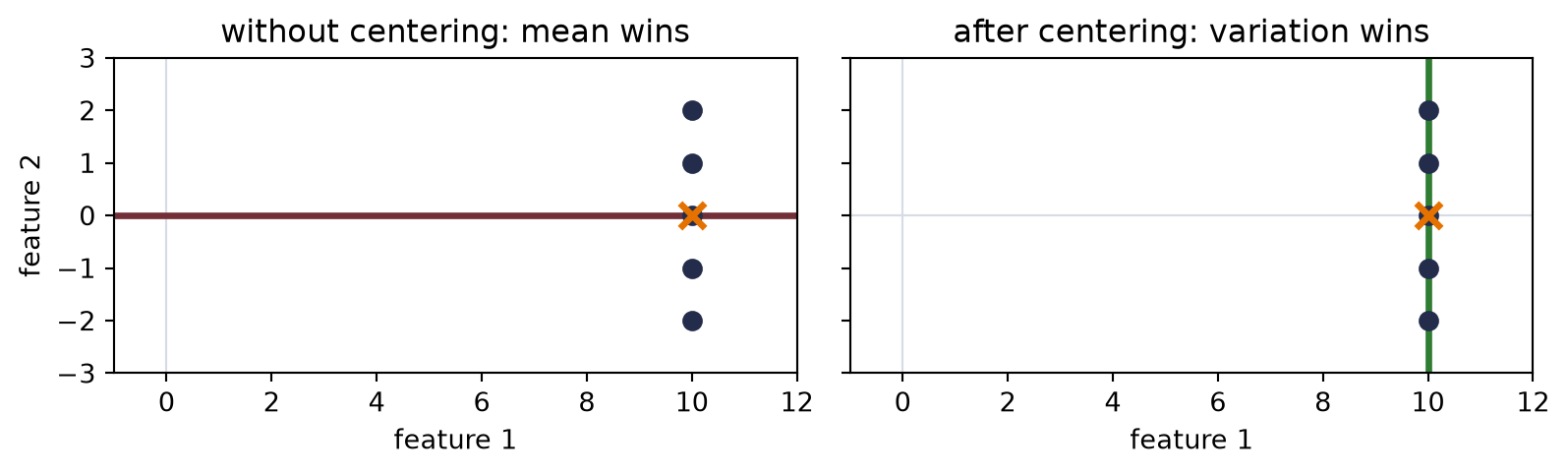
\[ \matr{Z}=\matr{X}_c\matr{V}_r, \qquad \widehat{\matr{X}} =\matr{Z}\matr{V}_r^{\top}+\vect{1}\vect{\mu}^{\top}. \tag{A.11}\]

For the usual sample-covariance convention, component \(i\) explains variance \(\sigma_i^2/(N-1)\). Centering is not cosmetic—it changes the question. Without it, the leading singular direction of the raw data matrix can mostly describe the offset from the origin.

The next five points all have first coordinate 10 and vary only in the second coordinate. What should PCA find? The answer is vertical variation. Raw SVD instead spends its first direction on the large mean; centering restores the intended question.

Figure code: make the PCA centering failure visible

observations = torch.tensor([
    [10.0, -2.0], [10.0, -1.0], [10.0, 0.0],
    [10.0, 1.0], [10.0, 2.0],
])
training_mean = observations.mean(dim=0)

_, raw_s, raw_vh = torch.linalg.svd(observations, full_matrices=False)
centered = observations - training_mean
_, centered_s, centered_vh = torch.linalg.svd(centered, full_matrices=False)

scores = centered @ centered_vh[:1].T
pca_reconstruction = scores @ centered_vh[:1] + training_mean
explained_variance = centered_s.square() / (observations.shape[0] - 1)
raw_values = [round(value, 6) for value in raw_s.tolist()]
centered_values = [round(value, 6) for value in centered_s.tolist()]

assert torch.allclose(raw_vh[0, 0].abs(), torch.tensor(1.0))
assert torch.allclose(centered_vh[0, 1].abs(), torch.tensor(1.0))
assert torch.allclose(observations, pca_reconstruction)

print("training mean:", training_mean.tolist())
print("uncentered singular values:", raw_values)
print("centered singular values:", centered_values)
print(f"uncentered top-axis |x alignment|: {raw_vh[0, 0].abs():.6f}")
print(f"centered top-axis |y alignment|: {centered_vh[0, 1].abs():.6f}")
print(
    f"centered rank-one max error: "
    f"{(observations - pca_reconstruction).abs().max():.3e}"
)
print("explained variance:", explained_variance.tolist())

fig, axes = plt.subplots(1, 2, figsize=(8.4, 3.6), sharex=True, sharey=True)
for axis in axes:
    axis.scatter(observations[:, 0], observations[:, 1], s=46,
                 color="#232D4B", zorder=3)
    axis.scatter(training_mean[0], training_mean[1], marker="x", s=90,
                 color="#E57200", lw=2.5, zorder=4)
    axis.axhline(0.0, color="#D6DCE5", lw=0.8)
    axis.axvline(0.0, color="#D6DCE5", lw=0.8)
    axis.set_xlim(-1.0, 12.0)
    axis.set_ylim(-3.0, 3.0)
    axis.set_aspect("equal")
    axis.set_xlabel("feature 1")

axes[0].plot([-1.0, 12.0], [0.0, 0.0], color="#722F37", lw=2.5)
axes[0].set_title("without centering: mean wins")
axes[0].set_ylabel("feature 2")
axes[1].plot([10.0, 10.0], [-3.0, 3.0], color="#2E7D32", lw=2.5)
axes[1].set_title("after centering: variation wins")
plt.tight_layout()
plt.show()

training mean: [10.0, 0.0]
uncentered singular values: [22.36068, 3.162278]
centered singular values: [3.162278, 0.0]
uncentered top-axis |x alignment|: 1.000000
centered top-axis |y alignment|: 1.000000
centered rank-one max error: 0.000e+00
explained variance: [2.5000000000000004, 0.0]

Two panels show five vertically aligned points at feature one equal to ten. Without centering, a horizontal axis from the origin is selected. After centering, a vertical axis through the orange mean marker follows all variation. — Figure A.3: PCA asks about variation around the training mean. These five points vary only vertically, but raw SVD first follows their large horizontal offset from the origin: its singular values are 22.360680 and 3.162278. After centering at (10, 0), the vertical singular value is 3.162278, the other is zero, and one component reconstructs every point exactly.

In a train/validation/test workflow, estimate \(\vect{\mu}\) and the principal directions on the training split only. Reuse that training mean for every later split; re-centering validation or test data separately changes the map and leaks information. The autoencoder interlude adds the next link: a tied linear autoencoder can recover the same principal reconstruction subspace under its stated centered, squared-loss, undercomplete, global-optimum conditions. It does not guarantee the same basis or that gradient descent reaches the optimum.

A.8 Practical `torch.linalg` checklist

When the algebra moves into code, ask these questions in order:

What are the last two dimensions? For operands with rank at least two, they define the matrix and leading dimensions are batches. Rank-one operands use matmul’s vector-specific insertion and removal rules; Appendix B works through those cases. Write the expected output shape before executing.
Is the task a product, a solve, or a least-squares problem? Use @, solve, or lstsq directly. Do not compute an inverse or pseudoinverse merely to multiply it by a right-hand side.
Does structure buy a better routine? Use eigh for real symmetric matrices and svdvals when only singular values are needed.
Are the values finite and the problem identifiable? Check finiteness, rank, conditioning, and residuals. A returned tensor is not evidence that the answer is trustworthy.
What is actually invariant? Compare reconstructions, losses, residuals, or projectors. Singular-vector signs and bases within repeated subspaces are not fixed.
Does autograd need the vectors? Gradients involving U or Vh can become unstable when singular values coincide or nearly coincide. If the objective needs only singular values, compute only those; otherwise test the gradient regime rather than assuming the forward decomposition settles it.

Okay, so—the whole appendix can be reduced to one habit: read the geometry and the shapes before trusting the operation. Matrices map one space to another; least squares projects onto what is reachable; SVD names the independent input and output directions; truncation has a precise norm guarantee; PCA adds the indispensable centering step. PyTorch will perform each calculation quickly, but it cannot decide whether you asked the right question.

Sources and further reading

Grant Sanderson, Essence of Linear Algebra: the visual interpretation of vectors, bases, and matrices as transformations. The figures here are independently constructed rather than adapted from the series.
Gilbert Strang, A Vision of Linear Algebra: input/output spaces, singular vectors, and the geometry of SVD in MIT OpenCourseWare.
Gilbert Strang, Linear Algebra 18.06SC: column spaces, projections, least squares, eigenvectors, and SVD.
Eckart and Young, The Approximation of One Matrix by Another of Lower Rank: the original low-rank approximation result; Mirsky later extended the norm statement.
Baldi and Hornik, Neural Networks and Principal Component Analysis: Learning from Examples without Local Minima: the qualified relationship between undercomplete linear autoencoders and principal subspaces used in the autoencoder interlude.
PyTorch, Linear algebra (torch.linalg): current interfaces for products, solves, decompositions, rank, and norms.
PyTorch, Numerical accuracy: conditioning, finite inputs, batched-operation differences, and spectral-decomposition caveats.

Exercises

(Pencil.) Let \(\matr{W}\in\mathbb{R}^{5\times3}\) be the weight of an nn.Linear(3, 5). Write the shapes of the output for inputs shaped \((3,)\), \((7,3)\), and \((4,7,3)\). Then explain why PyTorch evaluates a row batch with \(\matr{X}\matr{W}^{\top}\) even though the single-vector formula is \(\matr{W}\vect{x}\).
(Pencil and code.) From Equation A.3, derive \(\matr{X}^{\top}\vect{r}=\vect{0}\). Construct increasingly collinear design matrices, compare torch.linalg.lstsq(X, y) with a solve on the normal equations, and report residual and parameter error in float32 and float64. Do not assume which method first shows visible error.
(Pencil.) Using Equation A.6, prove Equation A.7. For a repeated singular value, show why rotating the corresponding columns of \(\matr{U}\) and \(\matr{V}\) together leaves \(\matr{A}\) unchanged.
(Code.) Generate a deterministic batch with shape \((6,8,3)\) and reconstruct all six matrices from reduced SVDs. Build rank-one and rank-two approximations, verify Equation A.10 for every batch member, and state a tolerance justified by the dtype and matrix scale.
(Code and interpretation.) Add a large offset to two-dimensional data and compare raw SVD with centered PCA. Fit the mean and basis on a training split; apply both unchanged to validation data. Compare projectors rather than signed basis vectors, and explain the leakage from recentering validation data.