3  Nonlinearity and the MLP

Chapter tools Lecture 1.1 · From Linear Regression to Neural Networks·Lecture 1.2 · Linear Regression via Neural Networks in Python·Download notebook·Open in Colab (opens in a new tab)

Our linear models can regress (Chapter 1) and classify (Chapter 2), and it is tempting to think we could get more power by simply stacking them: feed the output of one linear layer into another. Watch what happens:

\[ \matr{W}_2\bigl(\matr{W}_1\vect{x} + \vect{b}_1\bigr) + \vect{b}_2 = (\matr{W}_2\matr{W}_1)\,\vect{x} + (\matr{W}_2\vect{b}_1 + \vect{b}_2) = \matr{W}_{\text{new}}\,\vect{x} + \vect{b}_{\text{new}} . \tag{3.1}\]

The stack collapses. Two linear layers, or twenty, are exactly one linear layer with different knobs \(\rightarrow\) no amount of stacking buys any new expressive power. We need a nonlinear operation between the linear layers.

3.1 The four points a hyperplane cannot separate

You do not need messy real-world data to find the limits of a linear model. Four points on a flat plane suffice. The XOR function outputs 1 exactly when its two binary inputs differ:

\(x_1\)	\(x_2\)	XOR
0	0	0
0	1	1
1	0	1
1	1	0

Plot the four points and try to separate the 1s from the 0s with a single line. The positive examples sit on one diagonal, the negatives on the other; any line you draw puts at least one point on the wrong side. A linear classifier cannot represent this function, no matter how it is trained.

Why does a linear model fail here? Weight the four points equally. Each input on its own carries no evidence about the label: whether \(x_1\) is 0 or 1, the label is 1 half the time, and the same holds for \(x_2\), so the correlation between either input and the label is exactly zero. The label depends only on the interaction of the two inputs. A linear score \(\vect{w}^\top\vect{x} + b\) adds up the inputs’ separate contributions, so it has no term that could capture one.

NoteA historical scar: credit assignment, not just geometry

In 1969, Marvin Minsky and Seymour Papert published Perceptrons, proving that single-layer models cannot solve XOR. Folklore claims this mathematical limit killed early neural research, but the reality is subtler. Multilayer networks could already represent XOR; the open challenge was how to train them.

Without target labels for intermediate layers, how does an algorithm decide which hidden weight to blame for an output error? This is the credit assignment problem. Skepticism that it could be solved, alongside primitive hardware and funding cuts, stalled the field for over a decade. The barrier was never representation: it was the lack of an efficient learning rule. Backpropagation (Chapter 5) is that rule.

We confirm the linear model’s limit empirically: we train a linear model and a small MLP on the four points. The framework loop previewed in Chapter 1 does the training; Chapter 4 and Chapter 5 explain the optimizer and backward().

1. Fix the seed and write out the four XOR inputs and their labels.
2. Define the reusable train helper.
3. Run xor training.
4. Print the linear model’s probabilities and binary cross-entropy, then the MLP’s accuracy.

import torch
from torch import nn
torch.set_num_threads(4)  # pinned: results depend on the CPU thread count

# [1]
torch.manual_seed(6050)
X_xor = torch.tensor([[0., 0.], [0., 1.], [1., 0.], [1., 1.]])
y_xor = torch.tensor([0., 1., 1., 0.])

# [2]
def train(
    model: nn.Module, X: torch.Tensor, y: torch.Tensor,
    steps: int = 4000, lr: float = 0.5
) -> nn.Module:
    opt = torch.optim.SGD(model.parameters(), lr=lr)
    for _ in range(steps):
        opt.zero_grad()
        loss = nn.functional.binary_cross_entropy_with_logits(model(X).squeeze(-1), y)
        loss.backward()
        opt.step()
    return model

# [3]
linear = train(nn.Linear(2, 1), X_xor, y_xor)
mlp = train(nn.Sequential(nn.Linear(2, 4), nn.ReLU(), nn.Linear(4, 1)),
            X_xor, y_xor)

with torch.no_grad():
    linear_p = torch.sigmoid(linear(X_xor).squeeze(-1))
    linear_bce = nn.functional.binary_cross_entropy(linear_p, y_xor)
    mlp_acc = ((mlp(X_xor).squeeze(-1) > 0).float() == y_xor).float().mean()

# [4]
print(f"trained linear: probabilities {linear_p.numpy().round(3)}, "
      f"BCE {linear_bce:.3f}")
print(f" MLP (4 hidden): accuracy {mlp_acc:.0%}")

trained linear: probabilities [0.5 0.5 0.5 0.5], BCE 0.693
 MLP (4 hidden): accuracy 100%

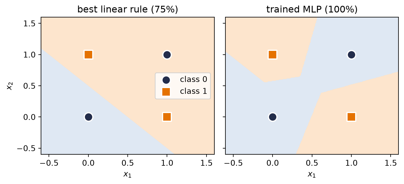
The trained linear model converges to the cross-entropy optimum for this symmetric dataset: it assigns a probability of exactly 0.5 to all four points, yielding a loss of \(\log 2 \approx 0.693\). The linear model’s logits differ from zero only by floating-point rounding, so thresholding them at 0 can report an apparent accuracy of 25%, 50%, or 75%; that number is a numerical artifact, not evidence of learning. Geometrically, any flat linear boundary can separate at most three of the four points (75%), whereas the four-unit ReLU network achieves 100%.

1. Build a dense grid of points around the four XOR inputs and open two side-by-side panels.
2. Decision regions.

import numpy as np
import matplotlib.pyplot as plt

# [1]
gx, gy = np.meshgrid(np.linspace(-0.6, 1.6, 220), np.linspace(-0.6, 1.6, 220))
grid = torch.tensor(np.stack([gx.ravel(), gy.ravel()], 1), dtype=torch.float32)

fig, axes = plt.subplots(1, 2, figsize=(7.4, 3.4), sharey=True)
# [2]
for ax, model, title in [(axes[0], None, "best linear rule (75%)"),
                         (axes[1], mlp, "trained MLP (100%)")]:
    with torch.no_grad():
        if model is None:
            Z = (grid.sum(1) - 0.5 > 0).float().reshape(gx.shape)
        else:
            Z = (model(grid).squeeze(-1) > 0).float().reshape(gx.shape)
    ax.contourf(gx, gy, Z, levels=[-0.5, 0.5, 1.5],
                colors=["#DCE6F2", "#FDE3C8"], alpha=0.9)
    for cls, marker, color in [(0, "o", "#232D4B"), (1, "s", "#E57200")]:
        pts = X_xor[y_xor == cls]
        ax.scatter(pts[:, 0], pts[:, 1], marker=marker, s=120, c=color,
                   edgecolors="white", linewidths=1.5, zorder=3,
                   label=f"class {cls}")
    ax.set_title(title); ax.set_xlabel("$x_1$")
axes[0].set_ylabel("$x_2$"); axes[0].legend(loc="center right")
plt.tight_layout(); plt.show()

Figure 3.1: Left: a representative best linear boundary gets three of four XOR points right, but one point must remain on the wrong side. Right: the trained 4-hidden-unit MLP carves separate regions for the two positive corners.

3.2 The neuron: a threshold with a hinge

Return once more to Figure 1.7. A neuron keeps that weighted-sum circuit and places a hinge directly at its output.

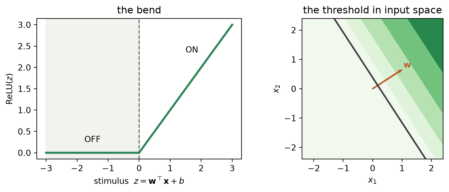
The artificial neuron takes its conceptual inspiration from biology: a cell integrates incoming signals and fires only when the accumulated stimulus crosses a threshold. Early models formalized this as a hard step function, but step functions have zero derivatives almost everywhere, which halts gradient descent. The modern, computationally friendly relaxation of that threshold is the rectified linear unit:

\[ \mathrm{ReLU}(z) = \max(0, z), \qquad f(\vect{x}) = \mathrm{ReLU}(\vect{w}^\top\vect{x} + b). \tag{3.2}\]

The affine combination \(\vect{w}^\top\vect{x} + b\) is the stimulus. Recall from Chapter 1 that it measures the similarity between the input and the template \(\vect{w}\), shifted by the bias \(b\). Below threshold, the neuron remains silent with an output of zero; above threshold, it fires with an intensity directly proportional to the stimulus.

1. Evaluate one neuron’s stimulus and rectified response.
2. Evaluate the same neuron over the input plane.

# [1]
z = torch.linspace(-3, 3, 300)
response = torch.relu(z)
# [2]
axis = torch.linspace(-2.4, 2.4, 220)
x1, x2 = torch.meshgrid(axis, axis, indexing="xy")
w, b = torch.tensor([1.0, 0.65]), -0.25
surface = torch.relu(w[0] * x1 + w[1] * x2 + b)

Figure 3.2: One neuron, two views. Left: the ReLU activation introduces a hinge at zero: silent on the negative half-line, linearly responsive on the positive side. Right: in the input plane, this cutoff defines a threshold hyperplane perpendicular to \(\vect{w}\); activation increases linearly as inputs advance into the active half-space.

Watch the mechanism: the cut never bends, the space does

XOR beats every straight line. Does fixing it need a boundary that curves?

The four rows of the XOR table above, carried through the neuron this figure draws: w = (1.0, 0.65) and b = −0.25. Hollow rings are the 0s, filled squares the 1s, and the third axis is that one neuron's own output.

\( \mathrm{ReLU}(z) = \max(0, z), \qquad \predictionpart{h} = \mathrm{ReLU}(\class{hl-stim}{\parameterpart{\vect{w}}^\top\featurepart{\vect{x}} + \parameterpart{b}}) \) \( \class{hl-cut}{\parameterpart{v_1}\featurepart{x_1} + \parameterpart{v_2}\featurepart{x_2} + \parameterpart{v_3}\predictionpart{h} + \parameterpart{v_0} = 0} \)

The cut never bent. The space did, and that is what one hidden unit buys.

The diagram is readable without playback. Opening this panel loads the optional controls.

One fixed drawing angle, not a three-dimensional view you can turn, and nothing here is trained: the chapter hands this neuron its w and b.

Scope and caveats

The XOR rows, the ReLU, the neuron and its weights are the chapter's; the rest is declared on this panel and solved from it. The swept fan of lines illustrates the chapter's "a hard linear boundary can classify at most three of the four points"; a fan of placements is not a proof, and the proof is the chapter's, not this picture's. The third axis is one neuron's activation — the same quantity the figure above contours — not a learned embedding dimension, and it is drawn at its own vertical scale, 0.7 drawing units per unit of activation, so heights are read from its ticks rather than against the two input axes. The cut is solved, not fitted: it is the unique plane whose four vertical clearances are equal, and they are equal because those four clearances always sum to the same 0.25 the rectifier clipped off at the origin. That cut uses all three coordinates, x₁, x₂ and h — the flat start of its tilt, a horizontal plane, is what a rule that kept only h would be, and it gets two of four; one neuron alone does not do XOR, and the chapter's next section builds boundaries out of several hinges. Inside the drawn window the final boundary reads as two separate straight pieces; they are two arms of one bent line whose corner lies well outside the frame, at x = (−2.07, 3.57). The drawn window, the swept fan, the flat starting plane and the camera are drawing devices; the four corners, their heights and every intersection are exact.

Check yourself. Keep w = (1.0, 0.65) but set b = 0, so every corner is ON. Could a flat cut still separate the lifted points?

No. With b = 0 the stimuli are 0, 0.65, 1.00 and 1.65 and nothing is clipped, so the heights are just a linear function of the inputs and all four lifted points lie on one plane: 0 + 1.65 = 0.65 + 1.00. The fold, not the third axis, is what separates them.

Transcript and keyboard help

1. Four XOR corners sit on a schematic input plane, seen from one fixed angle: hollow rings at (0,0) and (1,1) are the 0s, filled squares at (0,1) and (1,0) are the 1s. The chapter's own straight rule, x₁ + x₂ = 0.5, is drawn across them; the corner it gets wrong wears a wine ring and the readout says 3 of 4.
2. The line turns. The corner it gets wrong changes, and partway round two corners are wrong at once, so the readout falls to 2 of 4 and climbs back to 3. It never reads 4. The turn comes to rest with the line lying exactly along this neuron's own threshold, x₁ + 0.65x₂ = 0.25.
3. That resting line is now the neuron's, and it turns orange. One side is OFF, where the neuron is silent, and it is shaded; the other is ON. A weight arrow grows out of the line, pointing straight across it.
4. A third axis rises. The ON half of the plane tilts up into a sheet and each corner climbs to its own activation: 0.00, 0.40, 0.75 and 1.40. The OFF corner at (0,0) stays pinned flat at zero, because the rectifier clipped it.
5. A hollow ghost drops out of that pinned corner to −0.25, the stimulus the rectifier threw away. Without the clip the four heights would be −0.25, 0.40, 0.75 and 1.40, and every one of them would lie on a single plane.
6. A flat plane arrives horizontal — a rule that reads the activation alone — and gets 2 of 4. It tilts, keeping perfectly flat, bringing the two input coordinates back in. At 3 of 4 the (1,0) square passes below it; at 4 of 4 the (0,0) ring passes above it, and the tilt stops.
7. Where that flat cut crosses the tilted sheet, a line is drawn in the air, and it falls to the input plane beneath it. A second piece of the boundary was already lying flat inside the OFF region.
8. The input plane now carries a two-piece boundary with the two 0 corners shaded off and the two 1 corners left in the band between them. The cut is still perfectly flat; the sheet under it is what bends.

Silent; paused initially; 1.5× playback. Focus the animation pane: Space or K plays/pauses, arrows seek between beats, Home/End jump, Escape pauses. The scrubber and speed menu also work by keyboard. Reduced-motion mode holds each beat's state instead of moving between them.

In one dimension, a single neuron turns a straight line into a hinge. In two dimensions, it divides the plane into a flat zero-floor and a rising ramp separated by a crease: an inactive half-space where the neuron stays silent, and an active half-space where it fires, with \(\vect{w}\) standing perpendicular to the dividing boundary. That threshold boundary is the elementary building block of everything that follows.

At the sharp corner \(z = 0\), the classical derivative is undefined. In theory, any slope in the subgradient interval \([0, 1]\) is valid. In practice, frameworks settle on a definitive convention by setting the derivative at zero to 0. Because exact zeros occur systematically with zero-initialized biases, sparse activations, and symmetric data, this choice is not a purely academic detail: it determines whether a unit at exactly \(z = 0\) receives any gradient. We analyze the gradient through this derivative in Chapter 5; Exercise 3 inspects units that stay permanently silent.

3.3 Layers of hinges: bumps and polytopes

One neuron makes one boundary. A layer of \(k\) neurons makes \(k\) boundaries. Their intersections partition the input space into convex polyhedral regions (bounded ones are polytopes), and within each region the layer computes a plain linear function. For fixed input dimension \(d\), the maximum region count of one generic hyperplane arrangement grows on the order of \(k^d\): polynomial in the width \(k\), and quadratic on a two-dimensional plane (Exercise 4 derives the exact count).

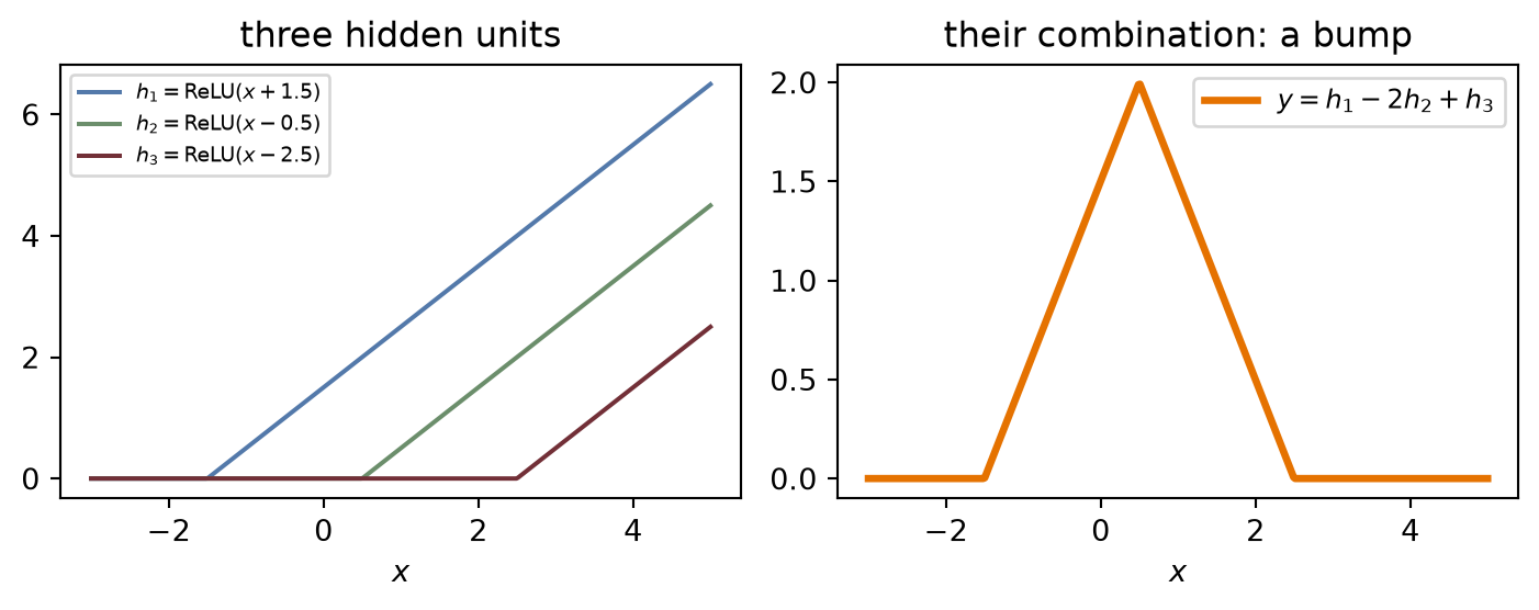
The simplest compact constructive example is one-dimensional. Combine three hinges so the slopes cancel again after the third breakpoint:

1. Combine three shifted hinges into a compact bump.

# [1]
xs = torch.linspace(-3, 5, 400)
h1 = torch.relu(xs + 1.5)
h2 = torch.relu(xs - 0.5)
h3 = torch.relu(xs - 2.5)
bump = h1 - 2 * h2 + h3

Figure 3.3: Three hinges make a compact triangular bump: the first starts the rise, the second reverses the slope, and the third cancels it back to zero. Bumps are the brush strokes of function approximation.

Watch the mechanism: three ramps that never come back down

Three ramps that never come back down — which middle coefficient brings their sum back to zero, to stay?

These three hinges are this chapter's hinge-bump-values cell, plotted just above. The panel adds them with one coefficient left free, c on the middle ramp. Every slope and sum it draws is computed from the cell; the chapter prints none.

−3 · steeper down+1 · a bare ramp

c =

−2

\( \displaystyle \predictionpart{g}(\featurepart{x}) = h_1 \: \class{hb-coef}{-2} h_2 + h_3 \)\( \displaystyle \predictionpart{g}(\featurepart{x}) = h_1 + \class{hb-csym}{c}\, h_2 + h_3 \)

Only −2 lands: slopes +1, −1, 0. Three endless ramps, one local bump.

The calculation is readable without playback. Opening this panel loads the optional controls.

Nothing here is learned: the three breakpoints and the three coefficients are placed by hand, as the chapter places them.

Scope and caveats

The chapter's coefficients are 1, −2, 1. That is why nothing on the picture is drawn in the colour reserved for a learnable parameter: the one control this panel has turns the middle coefficient by hand, in ink, and no optimizer ever touches it. The pale green shape standing from the first frame is the declared bump drawn ahead of its own construction — a target to aim at, not a second measurement — which is why it is the same green as the sum that aims at it; it stays while the control can still miss it, and only its dashed edge disappears, under the sum, when the sum lands. The control runs from −3 to +1 in steps of 0.25, and the timeline sweeps it from +1, a bare ramp, down to −2. Every sum drawn for a value other than −2, its three slopes +1, 1 + c, 2 + c, and the value 4.5 (2 + c) it reaches at the right edge are this panel's declared computed variants, not numbers of the chapter; the chapter writes one coefficient, −2, and one bump. The finished bump has four straight pieces, of slopes 0, +1, −1, 0; the ledger above the plot writes the last three and leaves the first, the flat zero before any hinge, to the picture. That −2 is forced rests on the equal spacing of the three breakpoints and on the outer coefficients both being 1: the last slope, 2 + c, and the height at the last breakpoint, 4 + 2c, vanish together only there. One bump is a construction, not an approximation theorem: how many hinges a given target needs, and whether training finds them, are the chapter's next questions and not this panel's claim.

Check yourself. Same three breakpoints. Which coefficients make the bump twice as tall?

2, −4, 2. Scaling every coefficient scales the whole function: the peak becomes 4 and the slopes 0, +2, −2, 0, so the sum is still exactly zero outside the window.

Transcript and keyboard help

1. Three hinges stand in one ink and three line styles — solid ReLU(x + 1.5), dashed ReLU(x − 0.5), dotted ReLU(x − 2.5) — each beginning at its own breakpoint and climbing at slope one for ever after, each named on top of its breakpoint's rule. Beside them, pale green, the finished bump already stands as a target, labelled bump. How could a sum of three such ramps ever make it?
2. A pen draws their plain sum on in green, from the left. As it crosses each breakpoint that ramp's coefficient, +1, is written beside its name and the slope of the sum on the piece that follows is written above the piece: +1, then +2, then +3. Each ramp adds its coefficient to the running slope, and the sum runs out of the top of the plot.
3. A hold. The middle coefficient is the one number the control under the picture turns; it stands at +1. Which value would bring the sum back to zero and keep it there? Decide before playing on — or drag the control and find out.
4. The coefficient sweeps down from +1. The dashed ramp, which is always c times h₂, swings down through the axis, and the sum's last two pieces swing with it: the middle piece about the apex, the tail about the axis. With too little the tail still climbs away; the sweep ends where the tail lies flat on zero.
5. It lands at −2, and only there: the ledger reads +1, −1, 0, because +1 − 2 + 1 = 0, and the sum lies on the target, whose fill deepens. The peak height 2 is written at the apex, which is g(0.5) = 2; a bracket under the ticks marks [−1.5, 2.5], the only place the sum is nonzero; the identity g(x) = h₁ − 2 h₂ + h₃ appears; and the ramps fade to a ghost. The four pieces, in order, have slopes 0, +1, −1, 0. Drag the control past −2 and the tail dives below zero for ever; stop short and it climbs away.

Silent; paused initially; 1.5× playback. Focus the animation pane: Space or K plays/pauses, arrows seek between beats, Home/End jump, Escape pauses. The scrubber and speed menu also work by keyboard. The c slider pauses playback and redraws the whole sum for its value; its arrow keys change c, not time, and it announces c, the three slopes and where the sum ends. Play or a timeline seek returns c to the recorded sweep. Reduced-motion mode holds each beat’s state: the sum is complete, and the coefficient stands at +1 or at −2, never in between.

Follow the pieces: before the first hinge, all units are silent and the output is zero. After the first breakpoint, \(h_1\) starts the climb. The coefficient \(-2\) on \(h_2\) reverses the slope at the peak, and \(h_3\) cancels that downward slope at the final breakpoint. Four linear pieces yield one compact bump.

3.4 The universal approximation theorem

Bumps are the whole secret. If you can make one bump, you can make many, at any position and height: with enough hidden units you can tile any continuous function, the way an artist paints a shape with brush strokes. That is the intuition behind the universal approximation theorem: a network with a single hidden layer can, in principle, approximate any continuous function on a closed and bounded region to any desired accuracy.

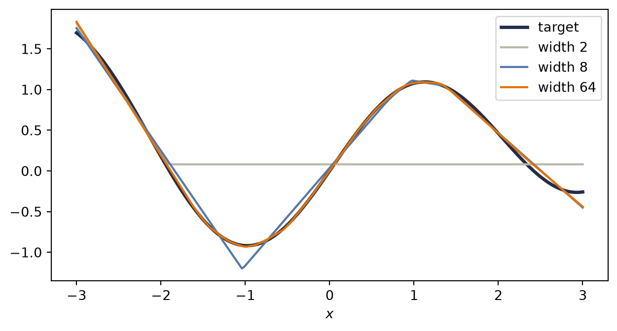
Fit one hidden layer at widths 2, 8, and 64:

1. Place 200 evenly spaced inputs on [-3, 3] and compute a sine-plus-quadratic target.
2. Define the reusable fit helper.
3. Implement the width sweep.

# [1]
xs1 = torch.linspace(-3, 3, 200)[:, None]
target = torch.sin(1.5 * xs1) + 0.08 * xs1 ** 2

# [2]
def fit(width: int, steps: int = 3000, lr: float = 0.05) -> torch.Tensor:
    torch.manual_seed(6050)
    net = nn.Sequential(nn.Linear(1, width), nn.ReLU(), nn.Linear(width, 1))
    opt = torch.optim.SGD(net.parameters(), lr=lr)
    for _ in range(steps):
        opt.zero_grad()
        ((net(xs1) - target) ** 2).mean().backward()
        opt.step()
    with torch.no_grad():
        return net(xs1).squeeze(-1)

plt.figure(figsize=(6.6, 3.6))
plt.plot(xs1, target, color="#232D4B", lw=2.5, label="target")
# [3]
for width, color in [(2, "#B8B8A8"), (8, "#5379AA"), (64, "#E57200")]:
    plt.plot(xs1, fit(width), color=color, lw=1.6, label=f"width {width}")
plt.xlabel("$x$"); plt.legend(); plt.tight_layout(); plt.show()

Figure 3.4: One hidden ReLU layer approximating a continuous curved target. Width 2 is too rigid; width 8 catches the shape; width 64 follows it closely. Width buys more hinge locations, but the theorem itself says nothing about where the optimizer places them.

The theorem guarantees less than beginners often assume:

WarningTrap: universal approximation is not a training guarantee

1. It does not tell you how to find the weights. Existence of a good network is not a training algorithm. Finding the weights is the job of the loss and the optimizer, and nothing guarantees gradient descent lands on the theorem’s solution.
2. It does not say the network is small. Tiling a complicated function with one-layer bumps can require astronomically many units.
3. In its usual uniform-approximation form, it speaks of continuous functions on closed and bounded regions and says nothing about how the fit behaves between or beyond your samples. A continuous ReLU network cannot uniformly approximate a jump to arbitrary accuracy: near the jump its worst-case error stays at least half the jump size. Under a mean-square (\(L_2\)) criterion, however, it can squeeze the transition into a narrow interval and make the average error arbitrarily small. The norm and the target class matter. Approximation is still not generalization; that distinction is the subject of Chapter 6.

3.5 Why depth: boundaries that bend

If one hidden layer suffices in principle, why is the field called deep learning? Efficiency, and geometry. A second hidden layer receives, as its inputs, the piecewise-linear outputs of the first; its boundaries are no longer straight lines. They fold wherever the first layer’s boundaries cut the space. Boundaries composed of boundaries: each layer folds the space the previous layer drew.

Concretely: a ReLU network is exactly linear inside each region of input space where the on/off pattern of its units is constant, and those regions are polytopes whose walls are the units’ boundaries. Deeper layers add walls that kink wherever they cross earlier ones. Exercise 4 has you draw this tiling and count its cells.

This folding compounds through repeated composition, and one dimension already shows how. A single hidden layer of \(k\) ReLU units cuts a line into at most \(k+1\) linear pieces, so the pieces grow linearly with width. Now let two units fold the interval \([0,1]\) into a tent, \(t(x) = 2\,\mathrm{ReLU}(x) - 4\,\mathrm{ReLU}(x - \tfrac{1}{2})\), which rises and then falls. Composing the tent with itself \(L\) times gives a sawtooth with \(2^L\) linear pieces from only \(2L\) units, because each fold doubles the pieces of everything beneath it. A single hidden layer needs \(2^L - 1\) units to match.

The same holds beyond one dimension: for suitable ReLU constructions at fixed input dimension, achievable region counts grow exponentially with depth, while a single hidden layer’s count grows polynomially with width. This is an existence construction, not a promise that gradient descent finds or uses all those regions. It is the economic argument for depth: deep networks fold space recursively and buy partitions that a shallow network would need exponentially more units to match.

3.6 Your first real MLP

We now build the model as a reusable class.

TipCoding hygiene: the house and its foundation

Every model you write from now on subclasses nn.Module, and the first line of your __init__ is always super().__init__(). Think of it as pouring the foundation before building the house: it is what wires up parameter tracking, .parameters(), and everything the optimizer and autograd need. Forget it and PyTorch raises an immediate exception, so the mistake is easy to find.

1. Register the hidden and output layers, then compose them in forward.

# [1]
class MLP(nn.Module):
    """A multilayer perceptron: linear layers with bends between them."""

    def __init__(self, input_dim: int, hidden_dim: int, output_dim: int):
        super().__init__()                      # the foundation
        self.hidden = nn.Linear(input_dim, hidden_dim)
        self.out = nn.Linear(hidden_dim, output_dim)

    def forward(self, x: torch.Tensor) -> torch.Tensor:
        return self.out(torch.relu(self.hidden(x)))

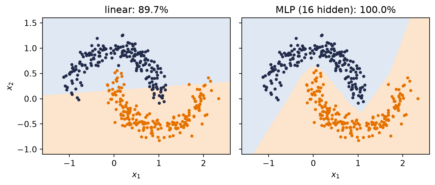
The problem is two interleaved moons, the classic shape no line can separate well. The training loop is unchanged; only the model is new:

1. Fix the seed, draw 200 noisy points on each of two interleaved moons, and reseed before fitting.
2. Fit a linear model and an MLP to the same moons.
3. Evaluate both decision rules on a dense grid.

# [1]
torch.manual_seed(6050)
n = 200
t = torch.rand(n) * torch.pi
moon1 = torch.stack([torch.cos(t), torch.sin(t)], 1) + 0.12 * torch.randn(n, 2)
moon2 = torch.stack([1 - torch.cos(t), 0.4 - torch.sin(t)], 1)
moon2 = moon2 + 0.12 * torch.randn(n, 2)
X_m = torch.cat([moon1, moon2])
y_m = torch.cat([torch.zeros(n), torch.ones(n)])

torch.manual_seed(6050)
# [2]
lin_m = train(nn.Linear(2, 1), X_m, y_m, steps=3000, lr=0.8)
torch.manual_seed(6050)
mlp_m = train(MLP(2, 16, 1), X_m, y_m, steps=3000, lr=0.8)

gx3, gy3 = np.meshgrid(np.linspace(-1.6, 2.6, 240), np.linspace(-1.1, 1.6, 240))
grid3 = torch.tensor(np.stack([gx3.ravel(), gy3.ravel()], 1), dtype=torch.float32)

# [3]
moon_panels = []
for model in (lin_m, mlp_m):
    with torch.no_grad():
        accuracy_value = (
            (model(X_m).squeeze(-1) > 0).float() == y_m
        ).float().mean()
        boundary_values = (
            model(grid3).squeeze(-1) > 0
        ).float().reshape(gx3.shape)
    moon_panels.append((accuracy_value, boundary_values))

Figure 3.5: Two moons: the linear model does what it can with one line (about 90% here); the MLP weaves its boundary through the gap and separates the classes completely.

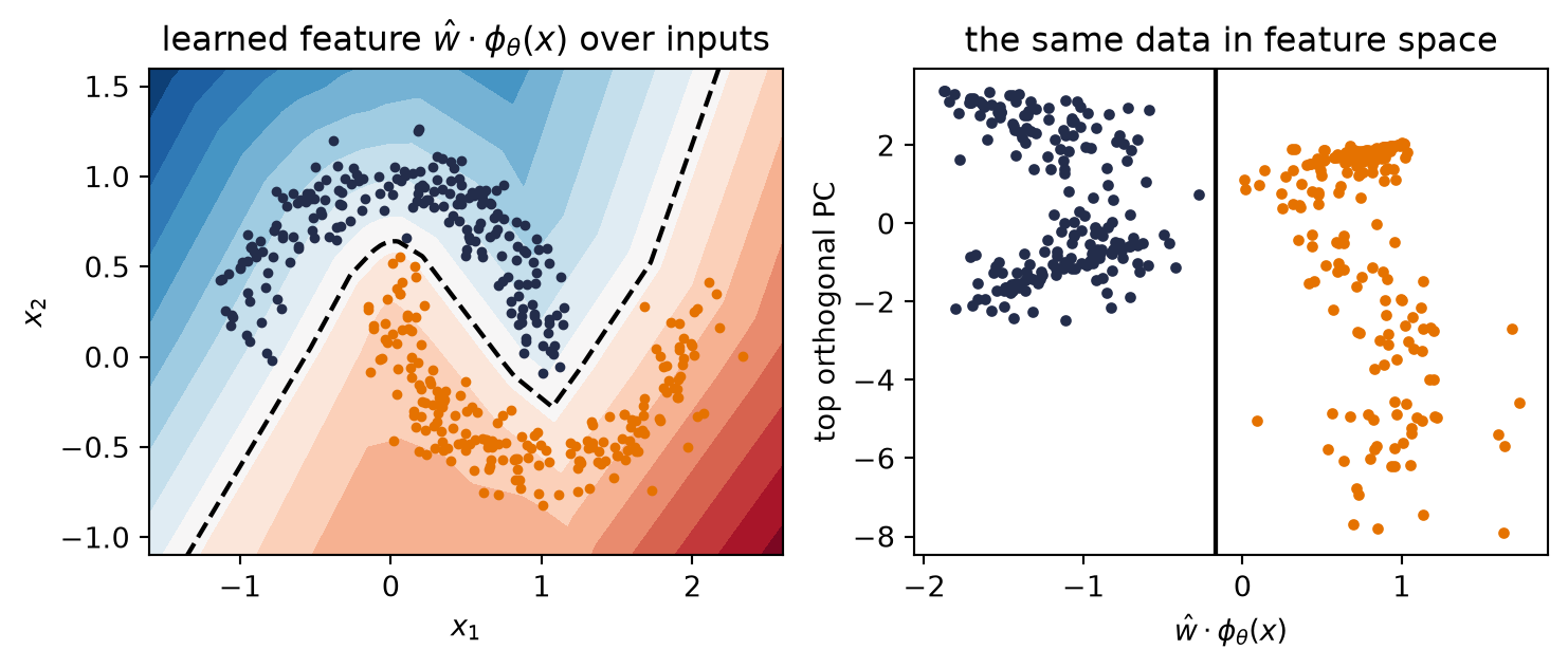
What happened to the curve? Nothing: the linear readout never had one. That distinction is the chapter’s central insight. The MLP did not learn a curved boundary; it learned a space in which the boundary is straight. Its readout is still a linear model, \(\vect{w}^\top \phi_\theta(\vect{x}) + b\): project the hidden activations onto the readout direction \(\hat{\vect{w}} = \vect{w}/\lVert\vect{w}\rVert\) and the decision boundary sits at the exact coordinate \(-b/\lVert\vect{w}\rVert\), a straight line. In Chapter 2’s vocabulary, the hidden layers form a backbone \(\phi_\theta\) and this readout is its classification head. Figure 3.6 visualizes this exact division: a linear readout operating on learned nonlinear features, with the moons plotted in the backbone’s coordinates.

1. Compute the hidden activations phi and their coordinate a1 along the unit readout direction.
2. Project the moons into learned readout and orthogonal coordinates.

# [1]
with torch.no_grad():
    phi = torch.relu(mlp_m.hidden(X_m))              # phi_theta(x): (400, 16)
    w = mlp_m.out.weight.squeeze(0)
    b = mlp_m.out.bias.item()
    w_hat = w / w.norm()
    a1 = phi @ w_hat                                 # readout coordinate
# [2]
    resid = phi - a1[:, None] * w_hat                # remove readout direction
    resid = resid - resid.mean(0)
    a2 = resid @ torch.linalg.svd(resid, full_matrices=False).Vh[0]
    boundary = -b / w.norm()                         # the line, exactly
    field = (torch.relu(mlp_m.hidden(grid3)) @ w_hat).reshape(gx3.shape)

Figure 3.6: The learned feature space, on the trained moons MLP from the previous figure. Left: the scalar feature \(\hat{\vect{w}}\cdot\phi_\theta(\vect{x})\) over the input plane; the dashed contour is the decision boundary, kinked wherever hidden units switch on or off. Right: the same points with coordinates (readout direction, top orthogonal principal component of \(\phi_\theta\)): the classes separate, and the boundary is the exact vertical line \(\hat{\vect{w}}\cdot\phi = -b/\lVert\vect{w}\rVert\). The network learns nonlinear features until a linear readout suffices.

Watch the mechanism: the space moves, the boundary does not

The MLP separates two moons that no single line can split. Did its boundary bend?

The figure above prints the start and the end side by side: the moons in the input plane, and the same points in the learned feature space. This is one schematic cloud carried continuously from the first picture to the second, with the readout's straight cut held still throughout.

\( \predictionpart{s}(\featurepart{\vect{x}}) = \parameterpart{\vect{w}}^{\top}\featurepart{\phi_\theta(\vect{x})} + \parameterpart{b} \) \( \class{fs-cut}{\hat{\parameterpart{\vect{w}}}^{\top}\featurepart{\phi_\theta(\vect{x})} = -\parameterpart{b}\,/\,\norm{\parameterpart{\vect{w}}}} \) \( \class{fs-bend}{\featurepart{\phi_\theta(\vect{x})}_i = \max(z_i, 0) + \lambda\min(z_i, 0)} \)

Grey paths show where the crossers began. Same points, same line, re-drawn space.

The diagram is readable without playback. Opening this panel loads the optional controls.

The cloud and the map are declared schematics: four fixed hidden units evaluated at a bend that opens, not a replay of the chapter's trained sixteen-unit network.

Scope and caveats

Nothing here is trained and no accuracy is claimed; the chapter's “about 90%” belongs to its own seeded run, whose points, \(\phi_\theta\) and boundary coordinate it does not print and this panel therefore does not reproduce. The moon shape is the chapter's own parametrisation sampled at sixteen equally spaced angles per moon with the radius alternating 1.07 and 0.93. The hidden weights and biases, the readout, and the second drawing direction are declared above and held fixed; only \(\lambda\), the slope on the negative side of the bend, moves, from 1 — where the layer is affine and the stack collapses, the chapter's first equation — to 0, the chapter's rectifier. Those intermediate bends are a drawing device for continuity, not an activation the chapter trains. Because the layer is the identity on the input plane in these two directions when \(\lambda = 1\), the first frame is the input plane itself, shifted; the horizontal coordinate is the readout coordinate at every \(\lambda\), so the cut at \(-b/\lVert w\rVert\) is one fixed line and the points, not the line, do the moving. The vertical coordinate is centred on the cloud's mean at every frame, as the chapter centres its residual before taking a principal component, and it is a declared orthogonal direction rather than the chapter's measured principal component. A straight cut in this feature space is a bent, piecewise-linear boundary back in the input plane — kinked wherever a hidden unit switches on or off, which is exactly the chapter's dashed contour and exactly the point. The convex hulls of the two declared classes overlap in the input plane, so the failure in the first frame is not a badly placed line: no straight line separates them there. Composition and reveal order follow the author's original animation.

Check yourself. Double every readout weight and the readout bias together, leaving the hidden layer alone. Does the cut move? Does the picture?

Neither moves. The drawn coordinate is \(\hat{w}\cdot\phi\), and \(\hat{w} = w/\lVert w\rVert\) is unchanged by scaling; the cut is \(-b/\lVert w\rVert = 1/4 = 0.25\), exactly what \(0.5/2\) already gave. Doubling the readout doubles every score and changes no decision.

Transcript and keyboard help

1. Thirty-two declared points, sixteen on each moon, in the input plane, with one straight cut drawn through them. Ten sit on the wrong side. Predict whether the cut has to bend.
2. The cut is not drawn by hand: it is the readout's own boundary, the exact coordinate minus b over the norm of w, which is 0.25 here. It will not move again.
3. The bend begins to open. Its negative-side slope lambda leaves 1, where the layer is affine and the whole stack collapses to one linear map, and the points start to move.
4. Each point travels a straight segment, because every drawn coordinate is affine in lambda. The cut stands where it stood, and it is still straight.
5. The two classes separate along the readout coordinate. Points cross the stationary cut one at a time, and the wrong-side count falls.
6. The last point crosses and the bend closes on lambda equal to zero: the chapter's rectifier, and the learned feature space of its figure.
7. The same straight cut now lies in a clear channel, with every point of both classes on its own side of it.
8. Grey paths recall where the ten crossers started. These are the same thirty-two points and the same straight line; only the space between them was re-drawn.

Silent; paused initially; 1.5× playback. Focus the animation pane: Space or K plays/pauses, arrows seek between beats, Home/End jump, Escape pauses. The scrubber and speed menu also work by keyboard. Reduced-motion mode holds each beat's state instead of moving between them.

For the XOR network, two hidden units suffice in principle, but such minimal networks are fragile; across random seeds they frequently get stuck at 50% accuracy with silent units (you will verify this in Exercise 3). A few spare units cost little and improve reliability. Chapter 4 will examine when optimization noise helps exploration; noise does not guarantee an escape.

3.7 A cautionary tale: representation without structure

Take image classification as an example. There is a seductive story often told about the hidden layers of a deep network: the first layer detects edges, the next combines them into textures and parts, and the next assembles objects, forming a tidy hierarchy of increasingly abstract features.

For a fully connected network on raw images, that is mostly not what happens. An MLP treats its input as one long, flat vector. In a dense weight matrix, neighboring pixels are no closer than pixels in opposite corners of the frame: the architecture encodes neither two-dimensional geometry nor locality, and nothing in it encourages a local-to-global hierarchy. Every unit connects to every pixel, so the first layer spends its parameters on diffuse, full-frame templates, and the parameter count explodes long before recognizable parts appear. The tidy hierarchy is not a property of depth itself; it appears in architectures that build locality in, and Part II builds one.

We now hold real expressive power: networks that can, in principle, approximate any continuous function on a closed and bounded domain. Universal representation does not guarantee sensible learning. What happens when an unconstrained model meets high-dimensional data whose geometry its architecture does not encode? Flexibility without inductive bias tends to fit coordinates rather than concepts. That missing structure has to come from the architecture, the data, and the training procedure.

NoteCheck yourself

Close the book for one minute and explain the hinge.

• Why does stacking linear layers without an activation still produce one linear map?
• What geometric object does one ReLU neuron introduce?
• How can a nonlinear feature map make a curved input-space problem linearly separable?

3.8 Okay, so: one hinge changed everything

1. Linear stacks collapse (Equation 3.1); XOR proves four points can defeat any line.
2. A neuron is a thresholded similarity score: below the boundary silent, above it proportional. One neuron yields one boundary; a layer forms a polyhedral partition; three hinges make a compact bump.
3. Bumps tile functions (universal approximation), but the theorem promises existence, not learnability, economy, or generalization.
4. Depth folds boundaries: suitable deep constructions can create region counts that grow exponentially with depth, yielding large efficiency gaps relative to comparable shallow constructions.
5. The MLP is a class now (nn.Module, foundation first), and it separates what no line can.

Sources and further reading

• Cybenko, “Approximation by Superpositions of a Sigmoidal Function” (1989) gives a foundational uniform universal-approximation result on compact domains.
• Hornik, “Approximation Capabilities of Multilayer Feedforward Networks” (1991) makes the distinction between uniform and \(L_p\) approximation explicit, which is exactly the jump-function nuance in this chapter.
• Nair and Hinton, “Rectified Linear Units Improve Restricted Boltzmann Machines” (2010) is an early empirical account of rectifiers preserving useful signal through multiple layers.
• Minsky and Papert, Perceptrons: An Introduction to Computational Geometry (MIT Press, 1969) is the rigorous analysis of single-layer perceptrons behind the historical callout.
• Minsky, “Steps Toward Artificial Intelligence” (1961) describes the credit assignment problem that hidden units pose for learning.
• Telgarsky, “Benefits of Depth in Neural Networks” (2016) gives the composed-tent construction whose \(2^L\) pieces a shallow network matches only with exponentially many units.
• Montúfar et al., “On the Number of Linear Regions of Deep Neural Networks” (2014) develops the architecture-dependent region-count argument behind the chapter’s case for depth.
• Lin, Tegmark, and Rolnick, “Why Does Deep and Cheap Learning Work So Well?” (2017) studies multiplication as a reusable compositional primitive and proves settings in which flattening that computation requires exponentially more units.

Exercises

1. (Pencil.) Generalize Equation 3.1: show by induction that any stack of \(L\) linear layers equals a single linear layer. Where exactly does inserting \(\mathrm{ReLU}\) between layers break your proof?
2. (Pencil.) Using the hinge construction, give explicit weights and biases for a one-hidden-layer network that outputs exactly 1 on \([0,1]\) and 0 outside \([-0.2, 1.2]\), a trapezoid. How many hidden units did you need?
3. (Code.) Retrain the XOR network with hidden_dim = 2 across ten different seeds. How often does it reach 100%? Inspect a failed run: what happened to its hidden units? (Hint: check how many are permanently silent.)
4. (Pencil.) For \(h\) lines in general position in two dimensions, derive the maximum region count \(1+h+\binom{h}{2}=\sum_{i=0}^{2}\binom{h}{i}\). (Code.) Color the input plane by ReLU on/off pattern for a random \(2 \to 8 \to 8 \to 1\) network initialized from a fixed seed. On successively finer grids, count the distinct activation patterns that appear (torch.unique(patterns, dim=0)). One pattern can occupy several disjoint cells; to count spatially connected cells, label connected components with scipy.ndimage.label. Compare with a parameter-matched wide network, \(2 \to 26 \to 1\): both have 105 parameters. Report the grid resolution with each count: a sampled count is a lower bound, not an exact count.
5. (Code.) Replace the moons MLP’s ReLU with nn.Identity() and retrain. Explain the resulting boundary in one sentence using Equation 3.1.
6. (Pencil.) Let \(\sigma\) be smooth and choose an offset \(c\) with \(\sigma''(c)\ne0\). Use Taylor expansion to show that \[ m_\lambda(u,v)= \frac{\sigma(c+\lambda(u+v))+\sigma(c-\lambda(u+v)) -\sigma(c+\lambda(u-v))-\sigma(c-\lambda(u-v))} {4\sigma''(c)\lambda^2} \longrightarrow uv \] as \(\lambda\to0\). (Code.) Use the logistic sigmoid with \(c=1\), sweep \(\lambda\) over \([10^{-6}, 1]\) on a logarithmic grid, and plot \(|m_\lambda(u,v)-uv|\) in float64 at \(u=0.6\), \(v=0.4\). Explain both the approximation-error regime and the eventual roundoff regime, and estimate the \(\lambda\) where they balance. Optional extension: compose seven of these approximate products into a balanced tree for \(x_1x_2\cdots x_8\); how does depth change the error, and how would you choose \(\lambda\) at each level? Named wrong answer: “expand the logistic sigmoid at \(c=0\)”; that is its inflection point, where \(\sigma''(0)=0\) and the proposed denominator vanishes.