Chapter 16 retained earlier keys and values so that each new query could form a weighted read. This interlude compares three ways to construct that memory computation: a query-local fit over stored pairs, running statistics for a factorized kernel, and an online linear predictor updated by the delta rule.
The constructions share a regression perspective, but they need not solve the same optimization problem. The kernel, predictor class, regularization, and update rule determine both the answer and the information that must be retained.
17.1 Three memory constructions through regression
The recurrent networks of Chapter 12 squeezed the evidence into a fixed-size state. The Transformer resolved that bottleneck by keeping all the visible evidence available. Its routing cost is quadratic in sequence length. There is another resolution: return to the regression perspective of Chapter 14 and change the kernel, the predictor class, or the update rule. Some of these choices permit a state of fixed size.
Recent sequence models make that move under names such as test-time regression, fast weights, linear attention, DeltaNet, and state-space sequence models. The names matter less than two questions about each solver: what does it keep, and what does it give up?
Choices within the regression framework
At time \(t\), let learned projections turn token representation \(\vect{x}_\tau\) into two views,
This is Wang, Shi, and Fox’s test-time-regression frame, written for vector values. The display specifies a reference fitting problem. An online update need not attain its minimizer. Query-local attention also makes the observation weights depend on the query, as the next construction shows.
Here the keys and values are computed from the input sequence. The memory state changes during the forward computation; the projection parameters are held fixed during that evaluation. The frame exposes four dials.
The views.\(W_Q,W_K,W_V\) are the learned projections of Chapter 15: queries and keys are compared, and values are what the comparison passes on. The token is not assigned one permanent meaning; the three projections give it a query, a key that provides the features used for comparison, and a value.
The history weights.\(w_{t,\tau}\) decide how much an older residual matters to the fitting problem. Chapter 12’s forget gates already made retention depend on time and content. A geometric schedule can privilege recent errors; an input-dependent schedule can keep some tokens longer than others.
The model and regularizer. The class \(\mathcal{M}\) decides whether the predictor is a local constant, a linear map, or something richer. \(\Omega\) brings back ridge penalties from Chapter 1 and weight decay from Chapter 4. Regularization controls the fitted map; it is not, by itself, the same operation as forgetting old observations.
The solver. A closed-form local fit, a running sufficient statistic, and one gradient step do different work and preserve different information. This is the new dial: what if the solver itself were a design choice, or even learned?
This objective is an umbrella, not an equivalence theorem. Its methods can restrict different function classes, use different weights, and stop at different approximations.
Solver 1: keep the data and fit at the query
Chapter 14 was more precise than saying “attention minimizes the shared objective.” For a query \(\vect{q}\), softmax attention solves the local-constant problem
Choose \(\kappa(\vect{q},\vect{k})=\exp(\vect{q}^{\top}\vect{k}/\sqrt{d_k})\) and the normalized coefficients are exactly a row of scaled dot-product softmax. The kernel supplies the weights; the constant fit supplies the average. An unrestricted \(M\) with unit observation weights and no regularizer would instead interpolate compatible training pairs and be undetermined away from them.
We can check numerically that the gradient vanishes at the weighted average. Subtracting the largest score rescales every \(\kappa_\tau\) by the same positive constant and leaves the minimizer unchanged.
Draw 12 seeded key-value pairs and a query, then form the weighted average, softmax output, and gradient.
This solver retains the key–value rows because a future query may weight every row differently. That is why dense causal attention carries a growing dataset forward.
Solver 2: collapse a factorized kernel into sufficient state
Suppose the kernel factors through a finite feature map \(\phi:\mathbb{R}^{d_k}\rightarrow\mathbb{R}^{r}\):
Assume the resulting kernel is nonnegative on the pairs being used and that the normalization denominator is positive. The positive feature map used below satisfies these conditions. Substitute that factorization into the weighted average and regroup terms:
The sufficient state is the pair \((\matr{S}_t,\vect{z}_t)\), not \(\matr{S}_t\) alone: the numerator needs accumulated value-weighted features and the denominator needs its normalizer. Each new pair updates that fixed-size state once. For this factorized kernel, any later query gets the same answer from the state as from a full traversal of all pairs.
Define the reusable ms_phi helper.
Initialize the sufficient-state pair, ms_S and ms_z, as zero arrays.
Compare a factorized-kernel traversal with its running state.
Check the claimed identities, shapes, or invariants.
Print whether ms_streaming matches ms_traversal and their largest absolute difference.
streaming equals traversal: True
max |difference|: 3.469e-17
The equality is exact up to floating-point order: the full dataset traversal has collapsed into two running sums. With \(r\) and \(d_v\) fixed, storage no longer grows with the prefix. Causal linear attention can therefore run as a recurrence: its state stores the sufficient statistics of this regression.
There is a price. Ordinary softmax’s exponential dot-product kernel does not have the finite exact feature map used above. With the scale \(1/\sqrt{d_k}\) absorbed into \(\vect{q}\), the kernel has the Taylor series \(\exp(\vect{q}^{\top}\vect{k})=\sum_{m\ge0}(\vect{q}^{\top}\vect{k})^{m}/m!\). Each power \((\vect{q}^{\top}\vect{k})^{m}\) is a dot product of features built from all products of \(m\) coordinates, as in \((\vect{q}^{\top}\vect{k})^{2}=\sum_{\ell,\ell'}(q_\ell q_{\ell'})(k_\ell k_{\ell'})\), so the series gives an exact feature map with such features for every \(m\), infinitely many in all. Changing to a finite factorization changes the kernel, or approximates it.1 Collisions in \((S_t,z_t)\) cannot be undone by revisiting a discarded row. The traversal equality is exact for the chosen factorized kernel, not a proof that finite-state linear attention reproduces exact softmax for arbitrary prefixes.
Solver 3: take one gradient step and get the delta rule
Now restrict the predictor to a scalar linear map \(M(\vect{q})=\vect{h}^{\top}\vect{q}\) and let the solver take one SGD step on only the newest pair. Its instantaneous loss and gradient are
Each outer product writes the residual left by the current key. Geometrically, the write changes the state only along that key, so a query orthogonal to the key reads the same value before and after the update. DeltaNet turns that classical online least-squares step into a sequence layer. The recurrence also exposes a state-space form: its transition is \(\matr{A}_t=\matr{I}-\eta_t\vect{k}_t\vect{k}_t^{\top}\) and its input write is \(\eta_t v_t\vect{k}_t\). The state transition is therefore determined by the current token’s learned key.
Where does forgetting enter? Exponential history weights \(w_{t,\tau}=\gamma^{t-\tau}\) define an exponentially weighted least-squares objective, but its exact minimizer generally requires a recursive least-squares covariance state. Writing \(\gamma\matr{H}_{t-1}\) into a one-step delta recurrence is a fading-memory solver choice, not an algebraic consequence of those weights. Gates can make that retention and the step size depend on the current token.
Such gates link this recurrence to the wider SSM family. Mamba makes parts of its state transition, input injection, and readout depend on the token; in the regression frame, those mechanisms play roles analogous to a learnable schedule for what to keep and what to write. Gated DeltaNet adds learned gating around delta-style updates. That reading is an analogy, not a claim that Mamba is literally obtained by differentiating the shared regression objective. Structured SSMs also use different state parameterizations and can cost less, in retained state and per-token work, than the dense outer-product recurrence here.
Retained state and per-token work
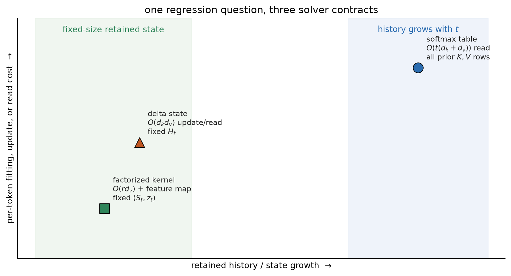
Figure 17.1: The solver map compares retained state and per-token work. Its positions are qualitative; the formulas and direct labels give the exact costs.
The asymptotic labels in Figure 17.1 describe this dense setup, not every implementation. Feature width \(r\), head dimensions, low-rank structure, convolutions, and hardware schedules change the constants and sometimes the order of growth.
WarningTrap: attention’s memory is a dataset, not a hidden box
Attention does not have a separate memory in the recurrent sense. The attention operation is the estimator; during causal decoding, the KV cache is the observed key–value dataset it must retain. A nonparametric query rule keeps growing data so it can form a new local fit. A parametric state instead compresses those data into a fixed-size object. FlashAttention changes how the uncompressed fit is scheduled; it does not compress the history into a fixed-size state. “Retains every row” does not mean “recalls every association exactly.” Softmax still returns a convex mixture whose quality depends on keys, temperature, and interference.
Mechanism test: recall under a fixed capacity
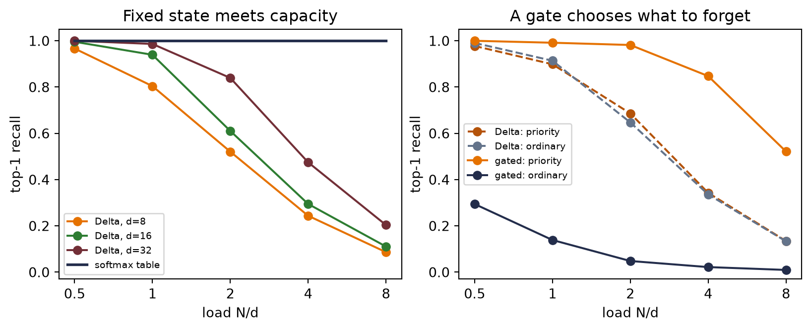
The storage comparison motivates a recall experiment: how does the one-pass delta update behave as more associations are written into a state of fixed dimension? We store \(N\) random unit key–value pairs, query every stored key, and decode each retrieved vector to the nearest stored value. Exact softmax attention keeps all pairs. A dense delta state has \(d^2\) numbers regardless of \(N\). A selective delta arm receives one extra priority bit and writes ordinary pairs at only one-tenth strength, so it can choose what to sacrifice.
We designed the study on two development seed branches. On those branches we fixed \(\eta=0.20\), the 25% priority rate, the 0.10 ordinary write gate, dimensions \((8,16,32)\), and loads \(N/d\in(0.5,1,2,4,8)\). Only then did we open the disjoint, held-out third branch for 30 endpoint repetitions. All methods in a trial receive the same keys, values, order, queries, and decoder. The endpoint code below is the frozen protocol; it runs on CPU in under a second on the reference machine.
Fix the seed, step size, ordinary write gate, three dimensions, five loads, and 30 repetitions.
Define the reusable helpers: ms_unit and ms_decode.
Define the reusable helpers: ms_trial and ms_panel.
Run the sealed synthetic recall-under-capacity study.
Figure 17.2: A sealed synthetic mechanism test. The uncompressed table keeps perfect top-1 identification in this sharp-softmax construction, while the fixed delta state loses associations as \(N/d\) grows. The selective arm receives a priority bit that the other arms lack and trades ordinary recall for priority recall. Keys, values, order, queries, decoder, and state width are matched; stored data, side information, and inference arithmetic are not.
At \(N/d=8\), the gate raises priority recall over the plain delta state by 0.387 on average and lowers ordinary recall by 0.124. The gate decides which pairs to lose, and total recall barely moves. Overall gated recall is 0.138 while plain Delta recall is 0.134 at that load. Given an extra signal, a fixed state can spend its capacity differently.
These results show interference under the specified delta update as the number of stored pairs grows. They do not establish a universal recall limit for fixed-size recurrent states. Now we can compare the three solvers. Keeping the dataset buys uncompressed access at growing cost; sufficient statistics buy an exact stream for a restricted kernel; online updates buy a steerable fixed state and accept interference. The RNN state has returned as one of these statistical choices.
NoteCheck yourself
Close the book for one minute and list what each solver keeps.
Which solver retains the original key–value rows?
Why does a factorized kernel need both \(S_t\) and \(z_t\)?
What information can a fixed delta state overwrite as its load grows?
17.2 Okay, so: the solver is part of the architecture
The objective alone does not specify the memory system. Views, history weights, function class, regularizer, and solver jointly define the result.
Softmax attention keeps a query-dependent dataset. It preserves every key–value row and pays a growing read cost.
A finite kernel feature map admits sufficient state. The pair \((S_t,z_t)\) reproduces the chosen factorized-kernel traversal without retaining raw rows.
One SGD step yields a delta update. Its fixed matrix writes residuals online, which makes capacity and interference explicit.
Selective retention spends a budget. The sealed recall study shows a gate trading ordinary recall for priority recall; it does not establish a universal architecture ranking.
(Pencil.) Starting from the local-constant objective, derive its stationarity equation and normalized solution. Identify exactly where the local-constant restriction enters. Why would an unrestricted function with no regularizer not imply the same average?
(Code.) Reproduce the factorized-kernel sufficient-state identity with a positive feature map of your choice. Assert that full traversal and the running pair \((S_t,z_t)\) agree for every prefix. Which assertion fails if you omit \(z_t\)?
(Pencil.) Derive the delta recurrence from one SGD step. Then multiply the old state by \(\gamma\). Explain why this is a fading-memory solver choice rather than the exact minimizer of exponentially weighted least squares.
(Code.) Sweep the capacity study over at least five state widths \(d\). Preserve the sealed-seed protocol, plot recall against both \(N\) and \(N/d\), and report where the curves align. Do not call top-1 identification exact value recall.
(Audit.) For each solver in the cost diagram, record state size, update cost, query cost, and information that cannot be reconstructed. Identify what is compute-matched and storage-matched, then design one matched test for a claim you would be willing to make.
We can cut the series off after an even power, which keeps the kernel positive, or use \(r\) positive features built from random projections, chosen so that \(\phi(\vect{q})^{\top}\phi(\vect{k})\) equals the kernel on average over the random draw (Choromanski et al.). In both cases the relative error can rise quickly as \(\norm{\vect{q}}\) and \(\norm{\vect{k}}\) grow.↩︎