12 Kernel Regression: Attention Before It Was Learnable

Chapter 11 ended with a machine that could translate, and one uncomfortable picture: every source fact had to cross a single fixed-size bridge before the decoder wrote its first token. The encoder had computed a state at every source position. Then we threw all but the last one away.

The lecture’s repair begins with an almost embarrassing question: why throw them away? Keep the whole sequence of encoder states as a memory bank. At each decoding step, ask what the decoder needs, compare that query with every stored state, and retrieve a weighted mixture of the relevant content. Keeping a bank does not make its entries lossless, but it removes the rule that all source information must pass through the last entry alone.

One problem remains: how should a query decide the mixture? A nearest-neighbor rule changes its chosen slot abruptly. We first need a smooth similarity-weighted rule, and statistics had one in 1964, half a century before modern neural attention.

Let us start with three observed pairs:

observation	location \(x_i\)	response \(y_i\)
1	1	1.5
2	3	2.8
3	5	1.8

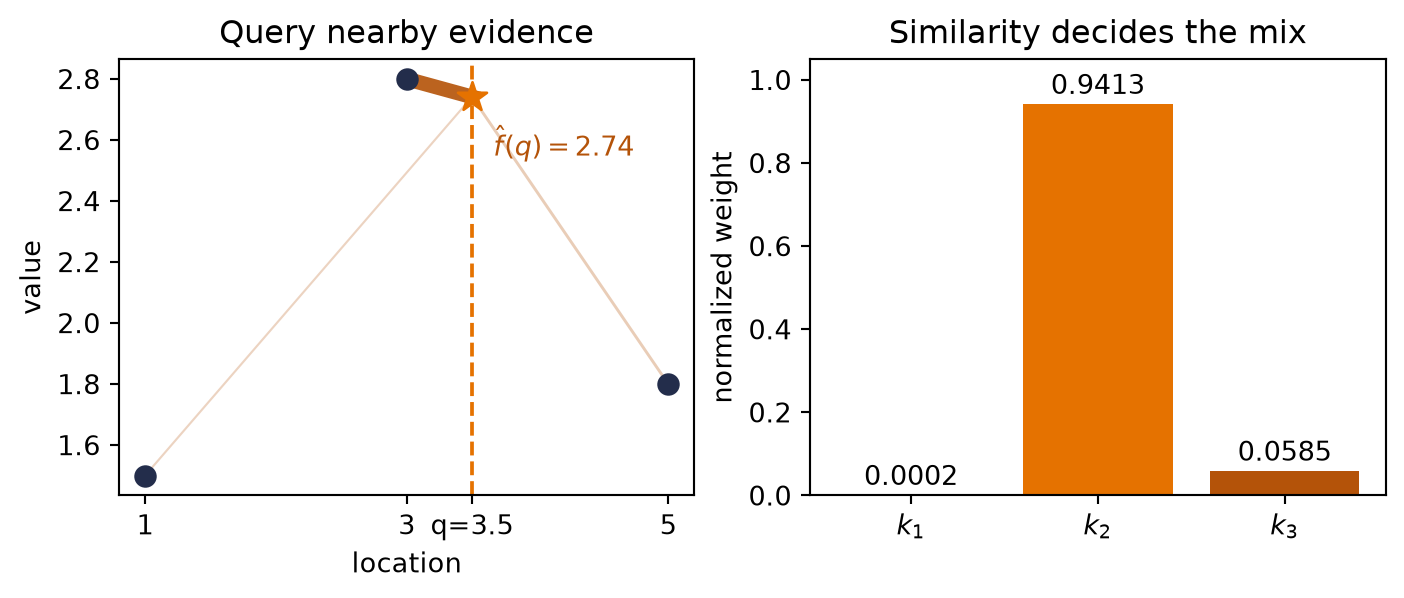
For a query \(q=3.5\), a Gaussian similarity with bandwidth \(h=0.6\) assigns weights \((0.0002, 0.9413, 0.0585)\). Their weighted mixture is \(2.7412\). The second observation dominates because its location is closest, the third contributes a little, and the distant first observation is nearly silent. No similarity function was learned; the chosen metric and bandwidth did the routing.

12.1 Chapter 1 already mixed old answers

There is a piece of unfinished business from Chapter 1. Linear regression makes a prediction by mixing the observed targets. It hid that fact inside the normal equation.

Let the augmented design matrix \(\widetilde{\matr{X}}\in\mathbb{R}^{n\times(d+1)}\) include the intercept column, let \(\widetilde{\vect{q}}\in\mathbb{R}^{d+1}\) be a new query with its leading 1, and let \(\vect{y}\in\mathbb{R}^{n}\) contain the observed targets. Assuming full column rank,

\[ \widehat{\vect{\beta}} = (\widetilde{\matr{X}}^\top\widetilde{\matr{X}})^{-1} \widetilde{\matr{X}}^\top\vect{y}. \]

The prediction at the query is therefore

\[ \widehat f(\vect{q}) = \widetilde{\vect{q}}^\top\widehat{\vect{\beta}} = \underbrace{\left[ \widetilde{\matr{X}} (\widetilde{\matr{X}}^\top\widetilde{\matr{X}})^{-1} \widetilde{\vect{q}} \right]}_{\vect{\lambda}(\vect{q})}^{\!\top}\vect{y}. \tag{12.1}\]

So Chapter 1’s promise was exact: \(\widehat f(\vect{q})\) is a weighted combination of the training targets. With an intercept, the weights sum to one because OLS reproduces a constant response. But weighted combination is not the same as weighted average. The entries of \(\vect{\lambda}\) may be negative.

For keys \((-2,-1,0,1,2)\) and query \(q=1.5\), the OLS weights are

\[ (-0.10, 0.05, 0.20, 0.35, 0.50). \]

They sum to one, yet the first is negative. If the targets are \((1,0,0,0,0)\), OLS predicts \(-0.10\), outside the observed range \([0,1]\). Linear regression is allowed to leave the observed targets’ convex hull even when the query lies inside the observed key range. For local smoothing, we want a stricter contract: nearby evidence should receive more weight, every weight should be nonnegative, and the weights should sum to one.

12.2 The magnifying glass becomes a kernel

A smoothing kernel is a similarity rule. It looks at a query and a stored key and returns a nonnegative affinity: large when they are close, small when they are far. To avoid confusing the kernel function with the matrix of keys later, we write it as \(\kappa_h\). The Gaussian choice is

\[ \kappa_h(\vect{q},\vect{k}) = \exp\!\left(-\frac{\norm{\vect{q}-\vect{k}}^2}{2h^2}\right), \qquad h>0. \tag{12.2}\]

The bandwidth \(h\) sets the width of the magnifying glass. A small value sees only the closest keys; a large value blends a broad neighborhood.

Given observed pairs \((\vect{x}_i,y_i)\), normalize the affinities,

\[ \alpha_i(\vect{q}) = \frac{\kappa_h(\vect{q},\vect{x}_i)} {\sum_{j=1}^{n}\kappa_h(\vect{q},\vect{x}_j)}, \qquad \widehat f_h(\vect{q})=\sum_{i=1}^{n}\alpha_i(\vect{q})y_i. \tag{12.3}\]

This is the Nadaraya–Watson estimator, proposed independently by Nadaraya and Watson in 1964. For the strictly positive Gaussian, each \(\alpha_i>0\) and \(\sum_i\alpha_i=1\). Scalar predictions remain between the smallest and largest observed values. Unlike OLS, this operator smooths locally while keeping every prediction inside the observed values’ convex hull.

The endpoint behavior is worth stating precisely. As \(h\to0^+\), the weight concentrates on the unique nearest key; exact nearest-key ties split the mass. At \(h=0\) the formula is undefined. As \(h\to\infty\), every finite distance looks alike and the weights approach \(1/n\).

Now let us make the lecture’s change of names. Locations \(\vect{x}_i\) become keys \(\vect{k}_i\), observed responses become values \(\vect{v}_i\), and \(\vect{q}\) remains the query. The formula does not change. Here is the whole operator in NumPy. The shapes come before the multiplication: queries are \((m,d)\), keys are \((n,d)\), values are \((n,p)\), and the returned mixture is \((m,p)\).

Code: fixed Gaussian attention, from scores to mixtures

from __future__ import annotations

import matplotlib.pyplot as plt
import numpy as np
import torch

torch.manual_seed(6050)
np.set_printoptions(precision=4, suppress=True)

def row_softmax(scores: np.ndarray) -> np.ndarray:
    """Normalize each row after a stability-preserving shift."""
    shifted = scores - scores.max(axis=1, keepdims=True)
    weights = np.exp(shifted)
    return weights / weights.sum(axis=1, keepdims=True)

def gaussian_attention(
    queries: np.ndarray,
    keys: np.ndarray,
    values: np.ndarray,
    bandwidth: float,
) -> tuple[np.ndarray, np.ndarray]:
    """Fixed Gaussian attention for Q:(m,d), K:(n,d), V:(n,p)."""
    if not np.isfinite(bandwidth) or bandwidth <= 0:
        raise ValueError("bandwidth must be positive and finite")
    if queries.ndim != 2 or keys.ndim != 2 or values.ndim != 2:
        raise ValueError("queries, keys, and values must be matrices")
    if queries.shape[1] != keys.shape[1] or keys.shape[0] != values.shape[0]:
        raise ValueError("Q/K feature dimensions and K/V row counts must agree")

    distances2 = ((queries[:, None, :] - keys[None, :, :]) ** 2).sum(axis=2)
    log_scores = -distances2 / (2.0 * bandwidth**2)  # (m, n)
    weights = row_softmax(log_scores)                # (m, n)
    return weights @ values, weights                 # (m, p), (m, n)

keys3 = np.array([[1.0], [3.0], [5.0]])
values3 = np.array([[1.5], [2.8], [1.8]])
query3 = np.array([[3.5]])
pred3, weights3 = gaussian_attention(query3, keys3, values3, bandwidth=0.6)
print("weights:", weights3[0])
print(f"prediction: {pred3.item():.4f}")

weights: [0.0002 0.9413 0.0585]
prediction: 2.7412

Figure: the three-point lookup

fig, axes = plt.subplots(1, 2, figsize=(7.2, 3.0), constrained_layout=True)
axes[0].scatter(keys3[:, 0], values3[:, 0], s=55, color="#232D4B", zorder=3)
axes[0].axvline(query3.item(), color="#E57200", ls="--", lw=1.4)
axes[0].scatter(query3.item(), pred3.item(), marker="*", s=130,
                color="#E57200", zorder=4)
for key, value, weight in zip(keys3[:, 0], values3[:, 0], weights3[0]):
    axes[0].plot([query3.item(), key], [pred3.item(), value],
                 color="#B45309", lw=0.8 + 5.0 * weight,
                 alpha=0.25 + 0.7 * weight)
axes[0].set(xlabel="location", ylabel="value", title="Query nearby evidence")
axes[0].set_xticks([1, 3, 3.5, 5], ["1", "3", "q=3.5", "5"])
axes[0].annotate(r"$\hat f(q)=2.74$", (query3.item(), pred3.item()),
                 xytext=(8, -22), textcoords="offset points", color="#B45309")

axes[1].bar(["$k_1$", "$k_2$", "$k_3$"], weights3[0],
            color=["#B0B7C3", "#E57200", "#B45309"])
for i, weight in enumerate(weights3[0]):
    axes[1].text(i, weight + 0.025, f"{weight:.4f}", ha="center")
axes[1].set(ylabel="normalized weight", ylim=(0, 1.05),
            title="Similarity decides the mix")
plt.show()

Figure 12.1: A fixed Gaussian lookup. The bars give the normalized weights, and the connecting lines show which observations feed the query. The query lands close to the second location, so its response dominates the mixture; no similarity function was learned.

The same code makes the OLS distinction concrete:

Code: signed OLS weights versus convex kernel weights

ols_keys = np.array([-2.0, -1.0, 0.0, 1.0, 2.0])
ols_query = 1.5
design = np.column_stack([np.ones_like(ols_keys), ols_keys])
query_design = np.array([1.0, ols_query])
ols_weights = query_design @ np.linalg.solve(design.T @ design, design.T)

witness_values = np.array([[1.0], [0.0], [0.0], [0.0], [0.0]])
nw_pred, nw_weights = gaussian_attention(
    np.array([[ols_query]]), ols_keys[:, None], witness_values, bandwidth=1.0
)
print("OLS weights:", ols_weights, "sum:", ols_weights.sum())
print("NW  weights:", nw_weights[0], "sum:", nw_weights.sum())
print(f"witness predictions: OLS {ols_weights @ witness_values[:, 0]:.4f}, "
      f"NW {nw_pred.item():.4f}; target range [0, 1]")

OLS weights: [-0.1   0.05  0.2   0.35  0.5 ] sum: 1.0
NW  weights: [0.001  0.0206 0.152  0.4132 0.4132] sum: 1.0
witness predictions: OLS -0.1000, NW 0.0010; target range [0, 1]

Which kernels make a convex average?

Only nonnegative smoothing kernels make this convex average. A Gaussian gives positive weights; a compact-support kernel may give zeros. Other objects also bear the name kernel. Equation 12.3 needs nonnegative numerators and a positive denominator.

12.3 Chapter 2’s scores-to-weights machine

Now harvest the second promise. Chapter 2 introduced softmax as the machine that turns arbitrary scores into nonnegative weights summing to one. Nadaraya–Watson has exactly that form. For any strictly positive kernel,

\[ \alpha_i(\vect{q}) = \frac{\kappa_h(\vect{q},\vect{k}_i)} {\sum_j\kappa_h(\vect{q},\vect{k}_j)} = \operatorname{softmax}_i\!\left( \log\kappa_h(\vect{q},\vect{k}_i)\right). \tag{12.4}\]

The score is the log-kernel. With the Gaussian,

\[ a_i(\vect{q}) = -\frac{\norm{\vect{q}-\vect{k}_i}^2}{2h^2}. \]

This also makes the temperature connection exact. If the unscaled score is \(s_i=-\norm{\vect{q}-\vect{k}_i}^2\), then

\[ \vect{\alpha}(\vect{q}) = \operatorname{softmax}\!\left(\frac{\vect{s}}{\tau}\right), \qquad \tau=2h^2. \tag{12.5}\]

Small bandwidth \(\rightarrow\) low temperature \(\rightarrow\) sharp lookup. Large bandwidth \(\rightarrow\) high temperature \(\rightarrow\) diffuse averaging. The factor \(2\) belongs to this score convention; if we had defined \(s_i=-\norm{\vect{q}-\vect{k}_i}^2/2\), the temperature would be \(h^2\) instead.

Notice the implementation never computes \(\kappa_h\) and then takes its logarithm. It computes the log-score directly, subtracts the largest score in each row, and only then exponentiates. That is Chapter 2’s stable-softmax hygiene, now paying rent again.

12.4 Bandwidth: the honesty gate

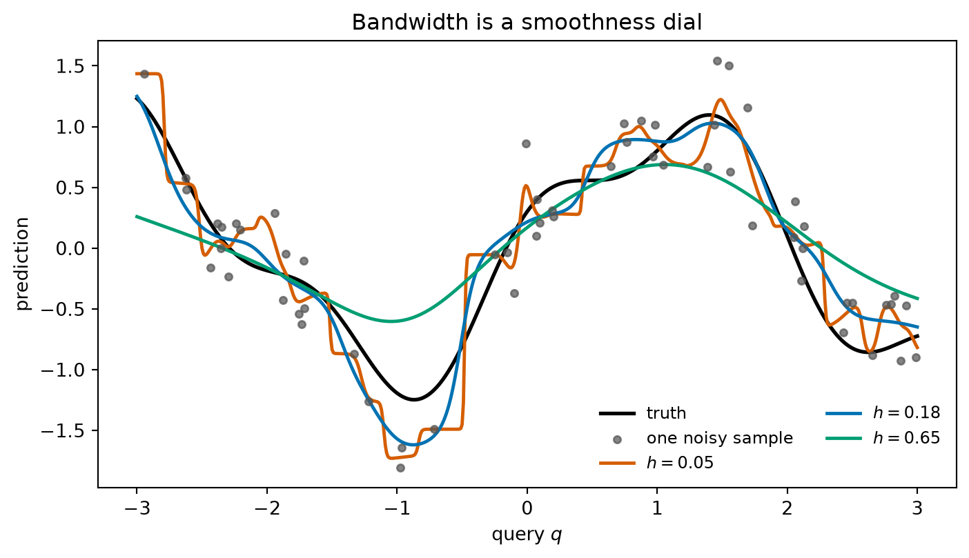
The three-point example makes a narrow bandwidth look wonderful. That is not evidence that narrower is better. A tiny neighborhood follows every noisy bump; a huge neighborhood washes real structure away. Chapter 1 called this bias versus variance. Here the bandwidth controls the trade.

Because this is a synthetic laboratory, we can do something ordinary observed data does not permit: hold 60 key locations fixed, redraw the response noise 1,000 times, and compare every prediction with the known function

\[ f(x)=\sin(1.5x)+0.3\cos(4x), \qquad y_i=f(x_i)+\epsilon_i, \qquad \epsilon_i\sim\mathcal{N}(0,0.25^2). \]

The key locations are seeded uniform draws on \([-3,3]\). The 241 query locations lie on \([-2.9,2.9]\) and share no exact coordinate with a key. Holding the design fixed lets us separate squared bias from variance over independent noise draws. The population identity

\[ \operatorname{MSE}=\operatorname{bias}^2+\operatorname{variance} \]

has no irreducible-noise term because we evaluate against the noiseless \(f\); predicting a fresh noisy response would add the irreducible variance \(0.25^2\) to every row. In our finite 1,000-world ensemble, the analogous empirical decomposition closes to floating-point roundoff.

Code: fixed-design bias/variance sweep over 1,000 noisy worlds

def truth(x: np.ndarray) -> np.ndarray:
    return np.sin(1.5 * x) + 0.3 * np.cos(4.0 * x)

data_rng = np.random.default_rng(605012)
keys = np.sort(data_rng.uniform(-3.0, 3.0, size=60))
observed_rng = np.random.default_rng(605013)
observed_values = truth(keys) + observed_rng.normal(0.0, 0.25, size=keys.size)
queries = np.linspace(-2.9, 2.9, 241)

mc_rng = np.random.default_rng(605014)
responses = truth(keys)[None, :] + mc_rng.normal(
    0.0, 0.25, size=(1_000, keys.size)
)
bandwidths = np.array([0.05, 0.08, 0.12, 0.18, 0.28, 0.42, 0.65, 1.00])

rows = []
for bandwidth in bandwidths:
    _, weights = gaussian_attention(
        queries[:, None], keys[:, None], observed_values[:, None], bandwidth
    )
    predictions = responses @ weights.T                 # (world, query)
    mean_prediction = predictions.mean(axis=0)
    squared_bias = np.mean((mean_prediction - truth(queries)) ** 2)
    variance = np.mean(np.var(predictions, axis=0))
    mse = np.mean((predictions - truth(queries)[None, :]) ** 2)
    rows.append((bandwidth, 2 * bandwidth**2, squared_bias, variance, mse))

print(" h     2h^2    bias^2  variance     MSE")
for row in rows:
    print(f"{row[0]:.2f}   {row[1]:.4f}   {row[2]:.4f}   "
          f"{row[3]:.4f}   {row[4]:.4f}")
best = rows[int(np.argmin([row[-1] for row in rows]))]
print(f"grid minimum: h={best[0]:.2f}, MSE={best[-1]:.4f}")

 h     2h^2    bias^2  variance     MSE
0.05   0.0050   0.0119   0.0343   0.0462
0.08   0.0128   0.0101   0.0247   0.0348
0.12   0.0288   0.0090   0.0169   0.0259
0.18   0.0648   0.0127   0.0109   0.0236
0.28   0.1568   0.0304   0.0069   0.0373
0.42   0.3528   0.0747   0.0047   0.0794
0.65   0.8450   0.1721   0.0031   0.1753
1.00   2.0000   0.3142   0.0022   0.3164
grid minimum: h=0.18, MSE=0.0236

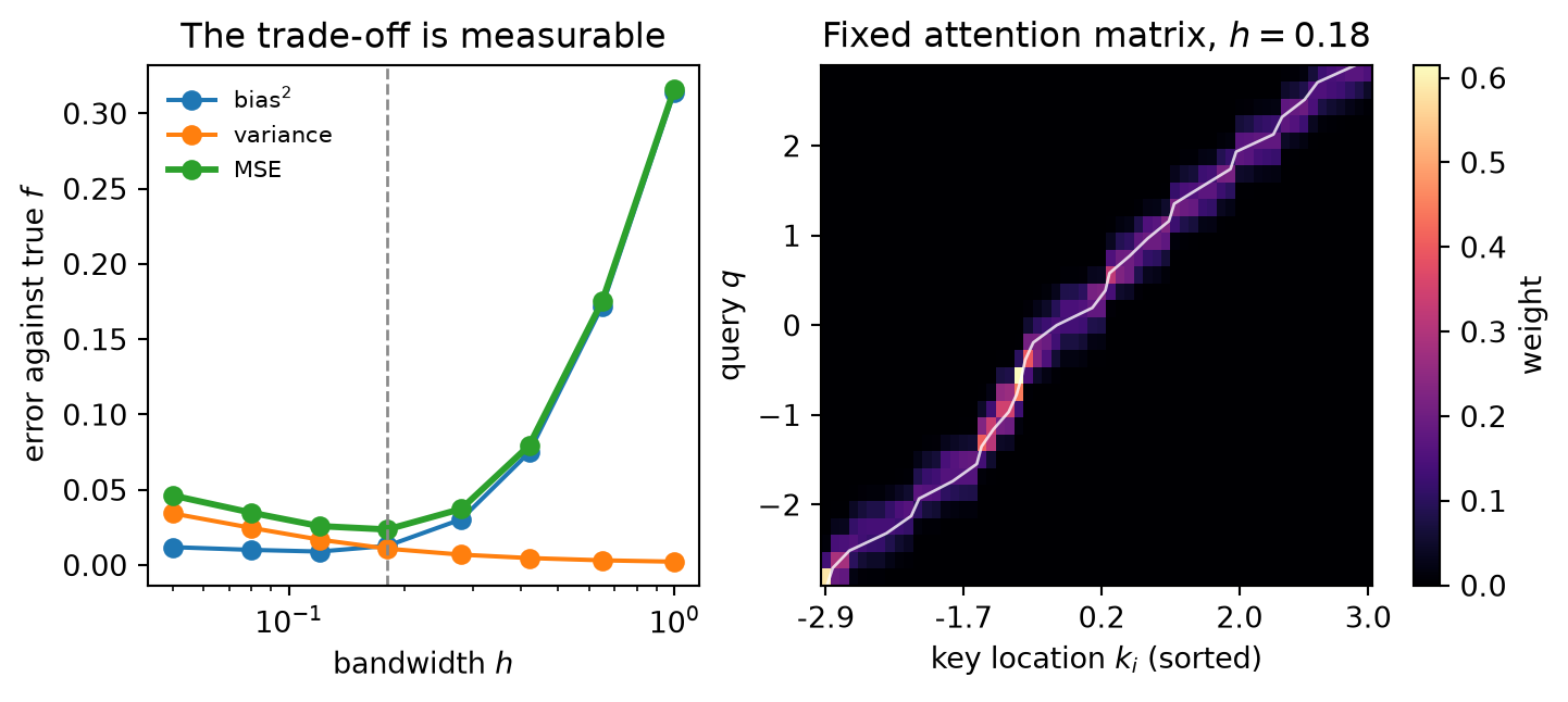
The variance falls at every step, from \(0.0343\) at \(h=0.05\) to \(0.0022\) at \(h=1.00\). Bias squared is not perfectly monotone at the sharp end of this sparse, random design; it bottoms at \(0.0090\) for \(h=0.12\), then rises to \(0.3142\) at \(h=1.00\). Their sum is the U-shaped quantity we care about. On this predeclared grid, \(h=0.18\) has the smallest MSE, \(0.0236\).

One noisy world shows what those numbers mean:

Figure: bandwidth as the smoothness dial

fig, ax = plt.subplots(figsize=(7.2, 4.1), constrained_layout=True)
dense = np.linspace(-3.0, 3.0, 601)
ax.plot(dense, truth(dense), color="black", lw=2.0, label="truth")
ax.scatter(keys, observed_values, s=15, color="#555555", alpha=0.72,
           label="one noisy sample", zorder=3)
for bandwidth, color in [(0.05, "#D55E00"),
                         (0.18, "#0072B2"),
                         (0.65, "#009E73")]:
    predictions, _ = gaussian_attention(
        dense[:, None], keys[:, None], observed_values[:, None], bandwidth
    )
    ax.plot(dense, predictions[:, 0], color=color, lw=1.8,
            label=fr"$h={bandwidth:.2f}$")
ax.set(xlabel="query $q$", ylabel="prediction",
       title="Bandwidth is a smoothness dial")
ax.legend(ncol=2, frameon=False, fontsize=9)
plt.show()

Figure 12.2: One fixed noisy sample under three bandwidths. The narrow rule follows local noise, the middle rule tracks the signal, and the broad rule erases the function’s smaller-scale structure. The blue bandwidth is the grid minimum in the 1,000-world audit, not a hand-picked attractive curve.

Selecting \(h\) when the truth is hidden

The known black curve is a laboratory privilege. On real data, choose the bandwidth using a validation set, then report once on a sealed test set. Training error alone will usually reward an extremely narrow kernel for copying each noisy target back to itself. The generalization protocol from Chapter 6 still applies even when nothing is trained by gradient descent.

12.5 From one query to an attention matrix

Now write the operator in the vocabulary that the rest of Part IV will keep. Let

\[ \matr{Q}\in\mathbb{R}^{m\times d},\qquad \matr{K}\in\mathbb{R}^{n\times d},\qquad \matr{V}\in\mathbb{R}^{n\times p} \]

hold \(m\) queries, \(n\) keys, and one \(p\)-dimensional value per key. The score and weight matrices are

\[ S_{ri}=-\frac{\norm{\vect{q}_r-\vect{k}_i}^2}{2h^2}, \qquad \matr{A}=\operatorname{rowsoftmax}(\matr{S}) \in\mathbb{R}^{m\times n}. \tag{12.6}\]

Every row of \(\matr{A}\) sums to one; columns generally do not. The pooled outputs are one matrix multiplication,

\[ \operatorname{Attention}_h(\matr{Q},\matr{K},\matr{V}) =\matr{A}\matr{V}\in\mathbb{R}^{m\times p}. \tag{12.7}\]

This is the book’s first attention-weight matrix. It is not a learned alignment. It is the allocation imposed by Euclidean distance and the chosen bandwidth.

Figure: measured trade-off and the first attention map

fig, axes = plt.subplots(1, 2, figsize=(7.4, 3.25), constrained_layout=True)
row_array = np.asarray(rows)
axes[0].plot(row_array[:, 0], row_array[:, 2], "o-", label=r"bias$^2$")
axes[0].plot(row_array[:, 0], row_array[:, 3], "o-", label="variance")
axes[0].plot(row_array[:, 0], row_array[:, 4], "o-", lw=2.2, label="MSE")
axes[0].axvline(best[0], color="#888888", ls="--", lw=1)
axes[0].set_xscale("log")
axes[0].set(xlabel="bandwidth $h$", ylabel="error against true $f$",
            title="The trade-off is measurable")
axes[0].legend(frameon=False, fontsize=8)

map_queries = np.linspace(-2.9, 2.9, 31)
map_predictions, attention_map = gaussian_attention(
    map_queries[:, None], keys[:, None], observed_values[:, None], best[0]
)
image = axes[1].imshow(
    attention_map, origin="lower", aspect="auto", cmap="magma",
    extent=(-0.5, len(keys) - 0.5, map_queries[0], map_queries[-1]),
)
key_index_at_query = np.interp(map_queries, keys, np.arange(len(keys)))
axes[1].plot(key_index_at_query, map_queries, color="white", lw=1.0, alpha=0.8)
ticks = np.array([0, 15, 30, 45, 59])
axes[1].set_xticks(ticks, [f"{keys[i]:.1f}" for i in ticks])
axes[1].set(xlabel="key location $k_i$ (sorted)", ylabel="query $q$",
            title=fr"Fixed attention matrix, $h={best[0]:.2f}$")
fig.colorbar(image, ax=axes[1], label="weight", fraction=0.05, pad=0.04)
plt.show()

print(f"Q {map_queries[:, None].shape}, K {keys[:, None].shape}, "
      f"V {observed_values[:, None].shape}, A {attention_map.shape}, "
      f"AV {map_predictions.shape}")
print("maximum row-sum error:",
      f"{np.max(np.abs(attention_map.sum(axis=1) - 1)):.2e}")

Figure 12.3: Left: the fixed-design bias–variance audit. Right: the same Gaussian rule written as a 31-query by 60-key attention matrix at \(h=0.18\). Bright cells receive more of a row’s unit mass; the white trace marks the \(k=q\) locus in sorted-key coordinates. The map is local and interpretable, but it was specified rather than learned.

Q (31, 1), K (60, 1), V (60, 1), A (31, 60), AV (31, 1)
maximum row-sum error: 2.22e-16

Read the bright band as a moving magnifying glass. Each query row reallocates one unit of weight across the stored keys. Where keys are dense, that unit is divided among several neighbors. Where keys are sparse, one or two slots carry most of it. Changing \(h\) changes the width of the band, exactly as changing temperature changes the spread of a softmax distribution.

There is one numerical trap. A Gaussian is mathematically positive everywhere, but a distant query and small bandwidth can make every directly exponentiated kernel value underflow to zero. Normalizing those zeros produces 0/0. The log-score version still has a largest entry, so the shifted softmax remains finite:

Code: verify the log-kernel identity and survive underflow

identity_query, identity_h = 0.37, 0.28
log_kernel = -0.5 * ((identity_query - keys) / identity_h) ** 2
direct_kernel = np.exp(log_kernel)
direct_weights = direct_kernel / direct_kernel.sum()
softmax_weights = row_softmax(log_kernel[None, :])[0]

far_log_kernel = -0.5 * ((1_000.0 - keys) / 0.1) ** 2
far_kernel = np.exp(far_log_kernel)
with np.errstate(divide="ignore", invalid="ignore"):
    naive_far_weights = far_kernel / far_kernel.sum()
stable_far_weights = row_softmax(far_log_kernel[None, :])[0]

print("max |normalize(K)-softmax(log K)|:",
      f"{np.max(np.abs(direct_weights - softmax_weights)):.2e}")
print(f"far query: naive denominator={far_kernel.sum():.1f}, "
      f"all finite={np.all(np.isfinite(naive_far_weights))}")
print(f"stable: sum={stable_far_weights.sum():.1f}, "
      f"nearest key={keys[np.argmax(stable_far_weights)]:.4f}")

max |normalize(K)-softmax(log K)|: 2.78e-17
far query: naive denominator=0.0, all finite=False
stable: sum=1.0, nearest key=2.9886

Similarity weights are not uncertainty probabilities

The entries of \(\matr{A}\) are probability-like allocations: nonnegative and row-normalized. They are not calibrated probabilities that the corresponding key is “correct,” and a sharp row is not automatically confidence. It may simply mean the bandwidth is small.

12.6 Return the fixed operator to the memory bank

The regression names now return to Chapter 11’s memory bank. Each one names a different job:

job	kernel regression	sequence memory preview
query	location \(\vect{q}\) where we need an answer	what the decoder needs now
keys	stored coordinates \(\vect{k}_i\)	descriptors used to match encoder memory slots
values	observed responses \(\vect{v}_i\)	content retrieved from those slots
weights	normalized fixed similarities \(\alpha_i(\vect{q})\)	how much each slot contributes
output	\(\sum_i\alpha_i\vect{v}_i\)	a query-specific context vector

Queries specify what is needed; keys provide what to compare against; values provide what to retrieve. In the simplest sequence model, the same encoder state can play both roles, just as our one-dimensional example stores a location and its response together. Later, learned projections will let keys and values carry different representations.

Chapter 1 also planted one more similarity primitive, the dot product:

\[ \vect{q}^\top\vect{k} =\norm{\vect{q}}\,\norm{\vect{k}}\cos\theta. \]

It is pure angular similarity only when the norms are controlled. If \(\vect{q}=(1,0)\), \(\vect{k}_1=(1,0)\), and \(\vect{k}_2=(2,0)\), both keys point in the same direction as the query, but their dot products are 1 and 2. Magnitude participates. That is not a defect; it is a reminder that the score defines what “similar” means.

Our score today is a hand-written negative squared Euclidean distance, and \(h\) is selected rather than learned. The operator stores the data, computes a fixed map, and pools the values. It shares attention’s normalized similarity-pooling algebra, but it has no learned compatibility function.

Now the Part II rhyme returns. Chapter 7 ended with a fixed image kernel and asked what would happen if the filter became learnable. Chapter 8 answered with a CNN. We end Part IV’s opening chapter with the same question:

What if the similarity itself were learnable?

The memory bank is ready. Query, keys, values, scores, row-wise softmax, and weighted pooling are ready. Only one hand-designed piece remains: the rule that decides whether a query and key belong together. Chapter 13 makes that rule learnable, then returns to Chapter 11’s date task so the decoder can show us where it looked.

12.7 Okay, so —

Chapter 1’s linear prediction already mixed training targets. OLS gives \(\widehat f(\vect{q})=\vect{\lambda}(\vect{q})^\top\vect{y}\), but its weights may be signed, so the prediction can leave the targets’ convex hull.
Nadaraya–Watson turns locality into a convex mixture. A nonnegative kernel scores query–key similarity; normalization makes the weights sum to one; their weighted values form the prediction.
Bandwidth is temperature in geometric clothing. For Gaussian distance scores, \(\tau=2h^2\): narrow is sharp and variable, wide is diffuse and biased. Our fixed audit reached its grid-minimum MSE of \(0.0236\) at \(h=0.18\).
Chapter 2’s softmax is the normalization exactly. Positive-kernel weights equal softmax(log kernel). Computing log-scores directly and shifting each row avoids the distant-query 0/0 trap.
Fixed attention is \(\matr{A}\matr{V}\). Queries score keys, row-softmax produces an \(m\times n\) allocation matrix, and that matrix pools the values. The algebra is complete; learning the score is the next chapter’s move.

Sources and further reading

Nadaraya, On Estimating Regression: the 1964 two-page paper introducing one side of the estimator now bearing Nadaraya and Watson’s names.
Watson, Smooth Regression Analysis: the independent 1964 development of smooth regression by local weighting.
Bahdanau, Cho, & Bengio, Neural Machine Translation by Jointly Learning to Align and Translate: the neural-attention step that replaces one fixed context with learned soft alignment; Chapter 13 performs that harvest.

Exercises

(Pencil.) Prove that Equation 12.3 is a convex combination when \(\kappa_h\ge0\) and its denominator is positive. Then prove that a scalar prediction lies in \([\min_i v_i,\max_i v_i]\). Which step fails for the OLS weights in Equation 12.1?
(Pencil.) For keys \((-2,-1,0,1,2)\), derive the five OLS target weights at \(q=1.5\) without using code. Verify that they sum to one, identify the negative weight, and construct a second target vector for which OLS leaves the target range.
(Code.) Split a fresh noisy sample from this chapter’s function into training, validation, and sealed test sets. Select \(h\) on validation data, report the test MSE once, and compare your selected curve with the synthetic-truth grid minimum above. Explain why the two procedures need not select the same bandwidth.
(Pencil + code.) Derive Equation 12.5. Then use keys \([0,0,1]\), query 0, and successively smaller positive bandwidths. What weights does stable softmax assign to the exact nearest-key tie, and why is \(h=0\) still invalid?
(Code.) Extend gaussian_attention to two-dimensional keys whose coordinates have very different units. Compare the attention map before and after standardizing each feature using training-set statistics. What does this reveal about the metric hidden inside a fixed kernel?