2  Linear Models that Classify: Logistic and Softmax

Chapter tools Lecture 1.1 · From Linear Regression to Neural Networks·Lecture 1.2 · Linear Regression via Neural Networks in Python·Download notebook·Open in Colab (opens in a new tab)

Regression predicts numbers; most of what the world wants predicted is categories: cat or dog, spam or not, which of ten digits. This chapter converts the linear machinery of Chapter 1 into a classifier without discarding a single idea: the same weighted sums, the same maximum-likelihood recipe for the loss, the same gradient descent. What changes is one squashing function at the output, and it changes less than you might think.

2.1 What actually changes

Return to the computation circuit in Figure 1.7. Keep every weighted input and the bias, but now call the circuit’s output a raw score \(o\). Classification adds one operation after that score; the weighted-sum machinery itself stays intact.

In regression, \(y \in \R\) and the Gaussian noise model handed us the MSE (Chapter 1). In classification, \(y\) is a label from \(\{0, \dots, K-1\}\). Could we just regress onto the labels with MSE anyway? We could, and it fails for a principled reason: the loss is a noise model, and Gaussian is the wrong model for a coin flip. A binary outcome deviates from its probability like a Bernoulli variable, not like additive Gaussian noise \(\rightarrow\) maximum likelihood demands a different loss.

What we need is two things:

1. a way to turn the model’s raw score (its logit, \(o \in \R\)) into a probability,
2. a loss that measures how wrong a probability is.

The linear map that produces those raw scores is the model’s head, here a classification head. It is the last layer, and its job is to turn whatever representation reaches it into task-specific logits.

2.2 Binary classification

From score to probability: the sigmoid

Our linear model produces \(o = \vect{w}^\top\vect{x} + b\), an unbounded score. The sigmoid squashes it into a probability:

\[ \sigma(o) = \frac{1}{1 + e^{-o}} . \tag{2.1}\]

1. Evaluate the sigmoid across a range of logits.

import torch
import matplotlib.pyplot as plt
torch.set_num_threads(4)  # pinned: results depend on the CPU thread count

# [1]
o = torch.linspace(-6, 6, 300)
sigmoid_response = torch.sigmoid(o)

Figure 2.1: The sigmoid maps any real score to \((0,1)\), crossing \(\tfrac{1}{2}\) exactly at \(o=0\) (left). In input space (right), that single score is the straight line \(\mathbf{w}^\top\mathbf{x}+b=0\) between the circles and the squares; the dashed contours \(\hat p = 0.1\) and \(0.9\) are parallel to it. Confidence grows with distance from the line, and the line itself never bends. Near the boundary \(\hat p\) stays close to \(\tfrac{1}{2}\); far from it, \(\hat p\) saturates toward 0 or 1.

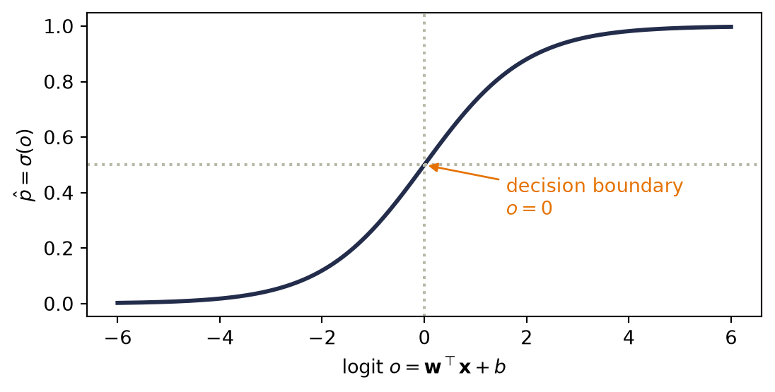
Watch the mechanism: crossing the line

One example walks across the decision boundary. What is its probability at the moment it touches the line — and does the next equal step buy as much?

The curve above, drawn over the same score range −6 to 6, read from the side the chapter does not draw: a small schematic input plane with a straight boundary, one tracked example x, its score o, and its probability \(\predictionpart{\hat p}\).

−6 · deep in class 06 · deep in class 1

score o =

+4.00

\( o = \parameterpart{\vect{w}^\top}\featurepart{\vect{x}} + \parameterpart{b} \) \( \predictionpart{\hat p} = \sigma(o) = \dfrac{1}{1 + \class{sq-tail}{e^{-o}}} \) \( \class{sq-zero}{o = 0} \iff \predictionpart{\hat p} = \class{sq-half}{\tfrac{1}{2}} \)

Two more equal pushes. The last buys 0.0294 — about an eighth of the first.

The calculation is readable without playback. Opening this panel loads the optional controls.

Nothing here is trained: the boundary is given, not learned, and the sigmoid is monotone, so it grades distance from that boundary without ever moving it.

Scope and caveats

The plane, its two labelled clusters, the weight vector and the bias are declared schematic geometry, not numbers this chapter prints; the sigmoid, its midpoint, the identity between a score of zero and a probability of one half and the score range −6 to 6 are the chapter's. A probability here is the model's output, not a measured frequency: no example on this plane has been counted. The score is the signed distance from the boundary times ‖w‖₂ = 2.5, so equal steps along the blue path are equal steps in o; the blue segment on the plane, the tick on the score axis and the point on the curve are one example seen three times, which is why they share a colour. Purple marks the labels y the clusters carry — squares for 0, discs for 1 — and the shapes, not the colour, carry that distinction. The score is the scene's one control; the timeline sweeps it and a drag is a detour.

Check yourself. Double every weight and the bias — take w to (3.0, 4.0) and b to −1.0. Where does the decision boundary move, and what happens to the probability at the point that scored 1?

The boundary does not move at all: doubling scales every score, so the set where the score is zero is the same straight line. But that point's score doubles to 2, and its probability rises from 0.7311 to 0.8808. Scaling sharpens confidence without bending the boundary.

Transcript and keyboard help

1. One example is tracked three times over: a blue dot on the class-0 side of the plane, a tick at o = −4.00 on the score axis, and a point on the sigmoid reading \(\predictionpart{\hat p}\) = 0.0180.
2. It moves straight along the boundary's normal toward the line. The score rises to −1.00 and the probability climbs to 0.2689.
3. Held one step short of the line. Predict the score and the probability at the line before releasing it.
4. Released; it slides the last step and comes to rest exactly on the boundary.
5. On the line the score is exactly 0 and the probability is exactly 0.5000. The dashed guides light up together: the boundary in the plane, o = 0 on the score axis, \(\predictionpart{\hat p}\) = ½ on the probability axis are one statement seen three times.
6. The first equal push: the example moves one step further along the same line, the score reaches 1.00 and the probability gains 0.2311.
7. The same push again. The score reaches 2.00 and this push gains only 0.1497.
8. Two more equal pushes, to 3.00 and 4.00, gaining 0.0718 and then 0.0294. The four marks on the probability axis crowd together while the four marks on the plane stay evenly spaced: equal steps in the score are not equal steps in the probability. Far from the line, the probability saturates toward 1.

Silent; paused initially; 1.5× playback. Focus the animation pane: Space or K plays/pauses, arrows seek between beats, Home/End jump, Escape pauses. The scrubber, the speed menu and the score slider also work by keyboard; the slider's own keys never move the timeline. Reduced-motion mode holds each beat's state instead of moving between them.

Notice what did not change: the decision boundary \(\hat{p} = \tfrac{1}{2}\) is exactly \(o = 0\), i.e. \(\vect{w}^\top\vect{x} + b = 0\), the same hyperplane geometry from Chapter 1, with \(\vect{w}\) still the template the input is scored against. The sigmoid does not bend the boundary; it grades our confidence on either side of it.

The loss: cross-entropy from maximum likelihood

Run the maximum-likelihood recipe with the correct noise model. If the labels are independent coin flips with \(P(y{=}1 \mid \vect{x}) = \hat{p}\), the likelihood of the dataset is \(\prod_i \hat{p}_i^{\,y_i}(1-\hat{p}_i)^{1-y_i}\); taking the negative log gives the binary cross-entropy:

\[ \loss_{\text{BCE}} = -\bigl[\, y \log \hat{p} + (1 - y)\log(1 - \hat{p}) \,\bigr]. \tag{2.2}\]

Read it as surprise: if the true label is 1, the loss is \(-\log \hat{p}\). It is small when the model believed in the outcome and explodes as that belief goes to zero. The more confidently wrong the model is, the larger the loss.

Watch the mechanism: the price of being sure and wrong

One example is truly labelled 1, and the model's belief in it slides toward zero. Equal steps down in belief — does every step cost the same?

The chapter's binary cross-entropy drawn as a picture: the belief \(\predictionpart{\hat p}\) along the bottom, the loss it buys up the side, and the (1 − y) branch drawn as the ghost it becomes once the label is hard.

0.01 · sure and wrong0.99 · sure and right

belief p̂ =

0.0125

\( \loss_{\text{BCE}} = -\bigl[\, \class{sl-live}{\targetpart{y} \log \predictionpart{\hat p}} + \class{sl-dead}{(1 - \targetpart{y})\log(1 - \predictionpart{\hat p})} \,\bigr] \) \( \targetpart{y} = 1 \;\Rightarrow\; \residualpart{\loss} = -\log \predictionpart{\hat p} \) \( \residualpart{\loss}\bigl(\tfrac{1}{2}\bigr) = \class{sl-hedge}{\log 2} \)

Every halving costs one more log 2. Belief can halve forever; the loss cannot stop.

The calculation is readable without playback. Opening this panel loads the optional controls.

Cross-entropy is not a distance and not a probability: the belief is bounded by 1, the loss is not bounded at all, and nothing here is trained.

Scope and caveats

The formula and the reading of it as surprise are the chapter's; the belief's journey and every loss value are declared computed variants, recomputed from that formula and never retyped. The logarithm is natural, so a loss is in nats — the chapter's information-theory reading of the same quantity comes later, and nothing here is called a bit. Only one term is ever active for a hard label: with y = 1 the second term carries the factor (1 − y) = 0, so the dashed curve is drawn to be dismissed, not read. A loss is not a probability and a probability here is not a measured frequency: no example has been counted and no model has been fitted. The loss ruler stops at 5 because a drawing must stop somewhere; the loss does not, which is the whole point. Nothing on this picture is orange, because nothing in this scene is a learnable parameter — the belief is handed to us, and where it comes from is the sigmoid one section above. The gradient of this loss, the prediction error itself, is the next section's business and is deliberately absent. The belief is the scene's one control; the timeline sweeps it and a drag is a detour.

Check yourself. Two examples, both labelled 1. Model A believes 0.50 on each. Model B believes 0.90 on one and 0.10 on the other — the same average belief. Which model's total loss is lower?

Model A, by a wide margin. Two hedges cost 0.6931 twice, 1.3863 in all. Model B pays 0.1054 for the belief of 0.90 and 2.3026 for the belief of 0.10, 2.4079 together — the one confident mistake costs more than both hedges. Averaging beliefs does not average the loss.

Transcript and keyboard help

1. One example, truly labelled 1, with a belief already in hand: \(\predictionpart{\hat p}\) = 0.9000. The wine arm under the curve is its loss, 0.1054. A second, dashed curve is the y = 0 term, which the factor (1 − y) = 0 switches off.
2. The belief falls in equal steps of 0.20, to 0.7000 and then 0.5000. The two risers measure what each step cost: 0.2513, then 0.3365. The treads are the same width; the risers are not the same height.
3. Halfway. The two curves cross here, so the loss is log 2 = 0.6931 whichever label is true — the price of admitting you do not know.
4. The same two steps again, to 0.3000 and 0.1000. Those risers are 0.5108 and 1.0986: the last equal step costs more than four times the first one did.
5. Held at 0.1000, loss 2.3026. Predict before releasing it: halving the belief to 0.05 — does that double the loss?
6. Released. The belief halves to 0.0500 and the arm climbs.
7. Not doubled: the riser is 0.6931, exactly log 2 and exactly as tall as the hedge. Halved again to 0.0250, and the riser is 0.6931 once more.
8. Halved a third time, to 0.0125 and a loss of 4.3820. Every halving buys the same 0.6931 while the belief step itself halves; the treads shrink to nothing and the risers do not.

Silent; paused initially; 1.5× playback. Focus the animation pane: Space or K plays/pauses, arrows seek between beats, Home/End jump, Escape pauses. The scrubber, the speed menu and the belief slider also work by keyboard; the slider's own keys never move the timeline. Reduced-motion mode holds each beat's state instead of moving between them.

The gradient with respect to the logit

Differentiate through the sigmoid and cross-entropy with respect to the logit (Exercise 1 walks you through the steps):

\[ \frac{\partial \loss}{\partial o} = \hat{p} - y . \tag{2.3}\]

The gradient is the prediction error, the same form MSE gave us for regression. All the logs and exponentials cancel. Softmax with cross-entropy gives the same cancellation.

2.3 Multiclass classification: softmax

With \(K\) classes, run \(K\) templates at once: \(\matr{W} \in \R^{K \times d}\) produces a score vector \(\vect{o} = \matr{W}\vect{x} + \vect{b}\), one logit per class.

TipThe first architectural block: the classification head

The linear map from an incoming representation to class scores is the classification head, also called a linear readout:

\[ \operatorname{head}(\featurepart{\vect{h}}) = \parameterpart{\matr{W}}\featurepart{\vect{h}} + \parameterpart{\vect{b}}, \qquad \parameterpart{\matr{W}} \in \R^{K \times d},\quad \parameterpart{\vect{b}} \in \R^{K}. \]

Its contract is narrow: take a \(d\)-dimensional representation \(\featurepart{\vect{h}}\), emit \(K\) logits \(\vect{o}\), and hand those logits straight to the loss. This chapter has no hidden layers yet, so the representation is the raw input, \(\featurepart{\vect{h}} = \featurepart{\vect{x}}\): here the whole model is the head.

Later models split into two parts. A backbone (also called the trunk) turns raw inputs such as pixels or tokens into a representation \(\featurepart{\vect{h}} = \phi_{\theta}(\featurepart{\vect{x}})\), and a small head reads the task’s answer off that representation. The backbone changes dramatically across the book, from multilayer perceptrons (Chapter 3) to convolutional stacks (Chapters 9 and 10) and Transformers (Chapters 16, 18, and 19); the head usually stays this small linear map. Because the two are separate, either can be swapped. Adapting a pretrained model to new classes often keeps its backbone and trains only a fresh head (Chapters 10, 18, and 20), and one backbone can feed several heads at once: a softmax head for a label beside a linear-regression head for a coordinate.

To turn \(K\) scores into a probability distribution, exponentiate (making everything positive) and normalize:

\[ \hat{y}_j = \mathrm{softmax}(\vect{o})_j = \frac{e^{o_j}}{\sum_{k=1}^{K} e^{o_k}} . \tag{2.4}\]

Softmax has three properties worth committing to memory: every output is positive, the outputs sum to one, and, less obviously, it is invariant to constant shifts: adding the same \(c\) to every logit changes nothing, because \(e^{o_j + c} = e^c e^{o_j}\) and the \(e^c\) cancels top and bottom. Only the differences between scores matter.

1. Compare softmax probabilities before and after a common logit shift.

# [1]
logits = torch.tensor([2.0, 0.5, -1.0, 1.0])
softmax_cases = [(shift, torch.softmax(logits + shift, dim=0))
                 for shift in (0.0, 100.0)]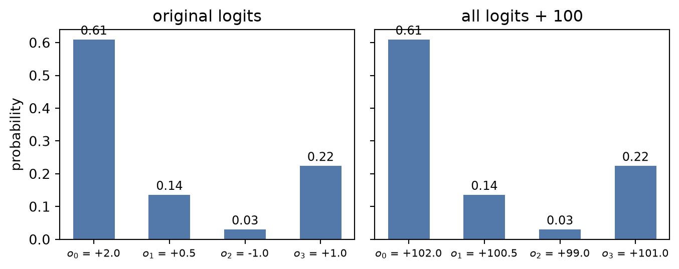

Figure 2.2: Softmax turns scores into a distribution. Shifting every logit by the same constant (right panel) leaves the probabilities unchanged: only the differences between scores carry information.

Watch the mechanism: the shift that changes nothing

Add 100 to every logit — which probability changes?

These four scores are this chapter's softmax-shift-audit fixture, and the figure above draws exactly these two cases. The figure rounds each probability to two decimals; this panel carries four.

\( \displaystyle \predictionpart{\hat{y}_j} = \dfrac{\class{sm-num}{e^{\featurepart{o_j}\class{sm-c}{{}+c}}}}{\class{sm-den}{\sum_k e^{\featurepart{o_k}\class{sm-c}{{}+c}}}} \) \( \displaystyle {}= \dfrac{\class{sm-ec}{e^{c}}\,e^{\featurepart{o_j}}}{\class{sm-ec}{e^{c}}\sum_k e^{\featurepart{o_k}}} \)

Back at c = 0: 0.6095, 0.1360, 0.0303, 0.2242 — the same four probabilities at every shift.

The calculation is readable without playback. Opening this panel loads the optional controls.

Softmax is invariant to adding a constant, not to scaling one: multiplying every score by a factor would change the distribution.

Scope and caveats

Only the common shift c moves, on the timeline rather than under a control. These probabilities are computed from four fixed scores: no training, no data, and no learnable parameter, which is why nothing here is drawn in the colour reserved for one.

Check yourself. Subtract the largest logit, 2.0, from all four. What are the new logits, and what happens to the probabilities?

The logits become (0, −1.5, −3, −1) and the probabilities stay (0.6095, 0.1360, 0.0303, 0.2242): subtracting 2 is adding the constant −2. This is the standard stability trick — the largest exponent becomes e⁰ = 1, so nothing can overflow.

Transcript and keyboard help

1. Four fixed scores: o₀ = 2.0, o₁ = 0.5, o₂ = −1.0, o₃ = 1.0. Before playing: after adding 100 to every one of them, which probability changes?
2. Exponentiate: the four exponentials are 7.39, 1.65, 0.37 and 2.72, sharing the sum 12.12. (Computed, as this chapter's landmine section prescribes, by subtracting the largest score first; the ratio is the same.)
3. Divide by the one shared sum: 0.6095, 0.1360, 0.0303, 0.2242, which add to 1.
4. Add c to every score, sweeping c from 0 to 100: the score ticks slide up together, the blue bars scale by the same factor, and the green bars stay on their c = 0 dashes. At c = 100 the ruler is relabelled 99 to 107 and the same marks stand where they stood: only the differences between scores matter.
5. Why: adding c to a score multiplies its exponential by one shared factor, and the same factor multiplies every term of the denominator, so it cancels top and bottom.
6. Return to c = 0: the same four probabilities, 0.6095, 0.1360, 0.0303, 0.2242; o₀ stays the largest throughout.

Silent; paused initially; 1.5× playback. Focus the animation pane: Space or K plays/pauses, arrows seek between beats, Home/End jump, Escape pauses. The scrubber and speed menu also work by keyboard. Reduced-motion mode holds each beat’s state: c snaps straight from 0 to 100 on the relabelled ruler for the shift and cancel beats and back to 0 for the last, never a value in between.

TipRemember this machine: scores \(\rightarrow\) weights

Step back from classification for a moment. Softmax is a differentiable way to turn a list of scores into positive weights that sum to one, giving larger scores more weight. Today the scores are class logits. Much later, we will score how well one current request matches several stored candidates, then use the resulting weights to blend what those candidates contain. For now, keep only the reusable machine: scores \(\rightarrow\) positive weights that sum to one.

NoteWhat “differentiable” buys us: softening the hard

Gradient descent cannot follow a cliff.

Consider the obvious way to pick a class: take the \(\operatorname{argmax}\), then output a one-hot vector with 1 at the winning index and 0 elsewhere. (The scalar \(\max\) operation is different: it passes a gradient through its winning input.) Argmax-plus-one-hot is hard. Nudge a losing logit slightly and the output does not move at all; nudge it past the winner and the output jumps all at once. Its derivative is zero almost everywhere, so the selection gives gradient descent no local hint about which losing score was close, which was far, or how the weights should change.

Softmax is a smooth relaxation of that one-hot selection; the name is literal: a soft max. Instead of crowning one winner, it spreads belief according to the scores, and every logit keeps a nonzero path to the loss. It is two things at once: a proper categorical distribution, the one cross-entropy scores below, and a smooth stand-in for a discrete choice. We gave up a little decisiveness and bought trainability.

A temperature \(\tau > 0\) sets how sharp or flat the softmax output is:

\[ \operatorname{softmax}(\vect{o}/\tau)_j = \frac{e^{o_j/\tau}}{\sum_{k=1}^{K} e^{o_k/\tau}} . \]

As \(\tau \to 0\) the distribution sharpens toward the hard winner; as \(\tau \to \infty\) it flattens toward uniform indifference; every value in between is smooth, so gradients reach every logit (Figure 2.3). If you have moved a “temperature” setting on a text generator, this is the same division: the generator divides its next-token logits by \(\tau\) and samples from the result. It is an entropy dial, not an imagination dial. Near \(\tau = 0\) sampling becomes greedy decoding, predictable and prone to repeating itself; at very large \(\tau\) it approaches uniform noise; in between, lower-ranked but plausible tokens occasionally win the draw.

Other discrete operations, such as a lookup, a yes/no branch, or even sorting a list (differentiable sorting exists), can be softened the same way: replace the hard decision with a smooth, temperature-controlled relaxation, train with gradients, and sharpen later if needed. We will need this relaxation for a hard memory lookup, where one address wins and every other row is ignored. In Part IV that single address becomes a softmax-weighted read across a whole bank of stored representations: the core of attention.

1. Compare one hard selection with three temperature-softened distributions.

# [1]
logits_demo = torch.tensor([2.0, 1.0, 0.2, -0.5])
klasses = ["A", "B", "C", "D"]
hard = torch.zeros(4); hard[logits_demo.argmax()] = 1.0
temperatures = [0.5, 1.0, 4.0]
soft_cases = [torch.softmax(logits_demo / temp, dim=0) for temp in temperatures]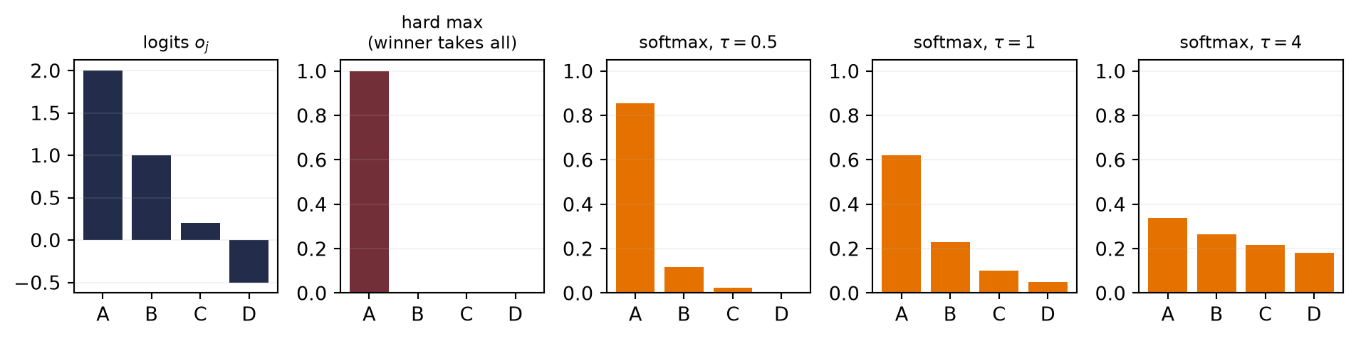

Figure 2.3: The softening move, in one row. The same four logits (left) pass through the hard argmax-plus-one-hot selection (a cliff with zero gradient almost everywhere) and through softmax at three temperatures. Small \(\tau\) sharpens toward the hard winner; large \(\tau\) flattens toward indifference; every version in between is smooth, so a useful derivative reaches every logit. Chapter 15 returns to this same normalization pattern.

Cross-entropy, multiclass edition

With one-hot labels \(\vect{y}\) (all zeros except a 1 at the true class), the cross-entropy is

\[ \loss_{\text{CE}} = -\sum_{j=1}^{K} y_j \log \hat{y}_j = -\log \hat{y}_{\text{true class}}, \tag{2.5}\]

the surprise at the true class, again. And the gradient has the same form:

\[ \frac{\partial \loss}{\partial o_j} = \hat{y}_j - y_j , \tag{2.6}\]

prediction minus target, one more time. This recurrence is no coincidence. The Bernoulli and categorical distributions belong to the exponential family, the logits are their natural parameters, and sigmoid and softmax, the inverses of their canonical links, map the logits back to the mean. Whenever a distribution of this family is paired with its canonical link, the model’s score is the natural parameter, and the gradient of the negative log-likelihood with respect to that score is the mean minus the observation, which is the prediction error.

NoteThe information-theory reading: coding and surprise

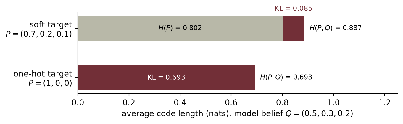
Probability and compression are two readings of the same objective. With natural logs, lengths are measured in nats.

• Entropy \(H(P) = -\sum_j p_j \log p_j\) is the uncertainty in a distribution: the shortest average code length possible for symbols drawn from \(P\).
• Cross-entropy \(H(P, Q) = -\sum_j p_j \log q_j\) is the average code length when symbols from \(P\) are encoded with a code built for the model’s belief \(Q\).

The gap between them is the Kullback–Leibler (KL) divergence, the extra length paid for using the wrong code:

\[ H(P, Q) = H(P) + D_{\mathrm{KL}}(P \,\|\, Q), \qquad D_{\mathrm{KL}}(P \,\|\, Q) = \sum_j p_j \log \frac{p_j}{q_j} \;\ge\; 0 . \]

A one-hot label puts probability 1 on the true class, so it has no uncertainty: \(H(P) = 0\). For one-hot labels, then, cross-entropy is the KL divergence, and both reduce to the surprise at the truth, \(-\log q_{\text{true}}\) of Equation 2.5. Minimizing this loss is at once maximizing the categorical likelihood, minimizing the expected code length, and minimizing the KL divergence from the labels to the model.

When the target is itself a soft distribution, \(H(P)\) no longer vanishes. If \(P\) is fixed, cross-entropy and KL still differ only by that constant; the distinction starts to matter when the first argument moves too, as in the alignment penalty of Chapter 21 and the variational autoencoder of Chapter 22. Appendix E compares KL with other ways to compare distributions.

Figure 2.4: Cross-entropy splits into the target’s own entropy plus the KL divergence, the extra code length paid for using the model’s belief \(Q\). The model belief is the same in both rows. A soft target (top) carries entropy of its own; a one-hot target (bottom) carries none, so its whole cross-entropy is KL divergence, the surprise \(-\log q_{\text{true}}\).

One numerical landmine

Computing \(e^{o_j}\) overflows once a logit exceeds roughly 88.7 in float32 (about 709 in float64), a scale training easily reaches. The fix exploits shift invariance: subtracting the maximum logit before exponentiating forces every exponent to be at most zero, which completely prevents overflow. This safeguard (the core of the log-sum-exp trick) changes nothing mathematically and everything numerically. We put it to work from scratch in the code below; Appendix C examines floating-point limits and hardware representations in depth.

2.4 Build it: three classes, from scratch

Now we assemble the full classifier on three Gaussian blobs. It has four pieces, all introduced in the preceding sections: three templates (one per class), the stable softmax, the cross-entropy loss, and the gradient. And since Equation 2.6 reduced that gradient to \(\hat{y} - y\), we can implement it by hand \(\rightarrow\) no autograd needed:

1. Fix the seed, draw three Gaussian blobs of 150 points each, and one-hot encode the labels.
2. Define the reusable stable_softmax helper.
3. Apply the softmax cross-entropy gradient to all three templates.
4. Print the final cross-entropy and accuracy on the training blobs.

# [1]
torch.manual_seed(6050)
centers = torch.tensor([[-2.0, 0.0], [2.0, 0.0], [0.0, 2.5]])
X = torch.cat([c + 0.7 * torch.randn(150, 2) for c in centers])   # (450, 2)
y = torch.arange(3).repeat_interleave(150)                        # (450,)
Y = torch.nn.functional.one_hot(y, 3).float()                     # (450, 3)

# [2]
def stable_softmax(logits: torch.Tensor) -> torch.Tensor:
    z = logits - logits.max(dim=-1, keepdim=True).values   # shift invariance at work
    e = torch.exp(z)
    return e / e.sum(dim=-1, keepdim=True)

W, b = torch.zeros(3, 2), torch.zeros(3)
# [3]
for step in range(400):
    P = stable_softmax(X @ W.T + b)          # (450, 3) predicted probabilities
    G = (P - Y) / len(X)                     # the beautiful gradient, eq. (6)
    W -= 1.0 * G.T @ X                       # residual out x signal in
    b -= 1.0 * G.sum(0)

P = stable_softmax(X @ W.T + b)              # evaluate the final updated parameters
ce = -(Y * torch.log(P)).sum(1).mean()
acc = (P.argmax(1) == y).float().mean()
# [4]
print(f"cross-entropy {ce:.3f}   accuracy {acc:.1%}")

cross-entropy 0.033   accuracy 98.9%

1. Score a dense grid with the trained classifier, then fill class regions and shade by confidence.
2. Overlay each class’s points and label the axes.

import numpy as np

# [1]
gx, gy = np.meshgrid(np.linspace(-4.5, 4.5, 300), np.linspace(-2.5, 5, 300))
grid = torch.tensor(np.stack([gx.ravel(), gy.ravel()], 1), dtype=torch.float32)
Pg = stable_softmax(grid @ W.T + b)
cls = Pg.argmax(1).reshape(gx.shape).numpy()
conf = Pg.max(1).values.reshape(gx.shape).numpy()

plt.figure(figsize=(6, 4.4))
plt.contourf(gx, gy, cls, levels=[-0.5, 0.5, 1.5, 2.5],
             colors=["#DCE6F2", "#FDE3C8", "#E3EEE3"])
plt.contourf(gx, gy, 1 - conf, levels=12, cmap="Greys",
             alpha=0.25, antialiased=True)
# [2]
for k, color in enumerate(["#232D4B", "#E57200", "#6B8E6B"]):
    plt.scatter(X[y == k, 0], X[y == k, 1], s=8, c=color, label=f"class {k}")
plt.xlabel("$x_1$"); plt.ylabel("$x_2$"); plt.legend(loc="lower right")
plt.tight_layout(); plt.show()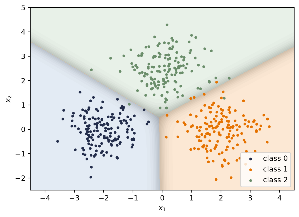

Figure 2.5: Three templates, three linear boundaries. Color shows the predicted class; shading shows confidence (the max softmax probability): crisp deep in each region, washed out along the boundaries where classes compete.

Replacing our manual loss with a framework’s built-in module takes just two lines, but conceals a classic trap. That loss object is the only new high-level tool introduced here: it scores logits against labels, while the manual loop above still supplies the parameter updates. Optimizers and automatic backpropagation stay black boxes, as in Chapter 1, until Chapters 4 and 5.

1. Create the framework loss object loss_fn from torch.nn.CrossEntropyLoss.
2. Compare the hand-computed cross-entropy with PyTorch’s fused loss.

# [1]
loss_fn = torch.nn.CrossEntropyLoss()
# [2]
print(f"ours: {ce:.6f}   torch: {loss_fn(X @ W.T + b, y):.6f}")

ours: 0.033425   torch: 0.033425

WarningLet PyTorch do the logits-to-probabilities conversion

nn.CrossEntropyLoss expects raw logits, and that is a feature, not a quirk: it fuses the softmax and the logarithm internally using the log-sum-exp trick, which is more numerically stable than any softmax-then-log you would write yourself. So the advice is: have your model output logits, hand them straight to the loss, and only apply softmax when you actually need probabilities to report. In PyTorch a classification head is simply an nn.Linear(d, K), and its contract is to emit raw logits \(\vect{o} \in \R^K\); it should not apply softmax internally. (The same goes for binary problems: prefer binary_cross_entropy_with_logits over sigmoid-then-BCE.) The classic bug is feeding softmax outputs into CrossEntropyLoss: the model still trains, just badly and silently. If a classifier is mysteriously mediocre, check this first.

NoteCheck yourself

Close the book for one minute and reconstruct the classifier.

• What remains linear before sigmoid or softmax is applied?
• Why does the target distribution determine the negative-log-likelihood loss?
• Why should logits, rather than already normalized probabilities, enter PyTorch’s cross-entropy loss?

2.5 Okay, so: classification is regression plus a normalizer

1. The linear geometry holds: logits are still template similarities \(\vect{w}^\top\vect{x} + b\), boundaries are still hyperplanes. Sigmoid and softmax grade confidence; here they act only on the output, not as nonlinear activations between layers. Applying an order-preserving function to the scores rescales certainty without folding space: every decision boundary remains an unyielding, rigid hyperplane. In the backbone-and-head vocabulary of the multiclass section, this whole model is a single classification head.
2. The loss came from the noise model, exactly as in Chapter 1: Bernoulli \(\rightarrow\) BCE, categorical \(\rightarrow\) cross-entropy, both read as surprise at the truth.
3. The gradient is the error, \(\hat{y} - y\), both times: the exponential-family pairing at work.
4. Softmax is a scores-to-weights machine, shift-invariant, numerically tamed by log-sum-exp; it will return, unchanged, as the normalizer of attention.

Next, we let the templates themselves be built out of other templates: Chapter 3 stacks these linear units into a backbone beneath the same head, and discovers why a nonlinear activation between them is not optional.

Sources and further reading

• Cox, “The Regression Analysis of Binary Sequences” (1958) develops the logistic model as a principled tool for binary outcomes.
• Bridle, “Probabilistic Interpretation of Feedforward Classification Network Outputs” (1990) connects normalized exponential outputs to probabilistic multiclass classification.
• Shannon, “A Mathematical Theory of Communication” (1948) is the original source behind the entropy and information vocabulary used to read cross-entropy.
• Kullback and Leibler, “On Information and Sufficiency” (1951) introduces the divergence that separates cross-entropy from entropy.
• Jaynes, “Information Theory and Statistical Mechanics” (1957) shows that the distribution with the most entropy at a given expected score has the exponential form of softmax.
• Blondel, Teboul, Berthet, and Djolonga, “Fast Differentiable Sorting and Ranking” (2020) is one example of replacing a hard, discrete operation with a trainable relaxation.

Exercises

1. (Pencil.) Derive Equation 2.3: write \(\loss_{\text{BCE}}\) as a function of \(o\) through \(\hat{p} = \sigma(o)\), use \(\sigma'(o) = \sigma(o)(1 - \sigma(o))\), and simplify. Which factors cancel, and why does this gradient never stall when the model is confident and wrong?
2. (Pencil.) Prove softmax’s shift invariance from Equation 2.4, then explain why subtracting the max logit makes the computation overflow-proof: what is the largest value ever exponentiated?
3. (Code.) Temperature: in Figure 2.3, scale the logits to \(\vect{o}/\tau\) for \(\tau \in \{0.05, 0.5, 1, 10\}\). Describe what happens to the distribution at both extremes, \(\tau \to 0\) and \(\tau \to \infty\), and connect each to greedy versus random decoding.
4. (Code.) Train the blobs classifier with MSE on one-hot targets instead of cross-entropy, using the per-example squared error summed over classes and averaged over examples. The manual loop needs a new logit gradient: row \(i\) becomes \(\frac{2}{n}\,\vect{p}_i \odot \bigl[(\vect{p}_i - \vect{y}_i) - \langle \vect{p}_i - \vect{y}_i,\, \vect{p}_i \rangle\bigr]\) (derive it, or check it against autograd). Compare convergence speed and the confidence shading near the boundaries. What does the wrong noise model cost?
5. (Code.) Increase the overlap between classes, either by raising the noise scale from 0.7 to 1.2 or by moving the blob centers closer, and retrain. Where does the confidence shading collapse, and what does the cross-entropy value tell you that the accuracy does not?
6. (Pencil.) Information-theory extension (optional). The temperature sets the balance between expected score and entropy. For logits \(\vect{o}\), a temperature \(\tau>0\), and any distribution \(P=(p_1,\dots,p_K)\) over the \(K\) classes, define \[ F(P)=\sum_{j=1}^{K}p_j o_j+\tau H(P). \] Let \(Q=\operatorname{softmax}(\vect{o}/\tau)\) and \(Z=\sum_{k=1}^{K}e^{o_k/\tau}\). Show that \(o_j=\tau(\log q_j+\log Z)\), and use it with \(\sum_j p_j=1\) to write \(F(P)=\tau\log Z-\tau\,D_{\mathrm{KL}}(P\,\|\,Q)\). Given that the divergence is never negative and is zero only when \(P=Q\), conclude that \(\operatorname{softmax}(\vect{o}/\tau)\) is the only distribution that maximizes \(F\). Set \(\vect{o}=\vect{0}\) to find the distribution with the most entropy. Which term of \(F\) dominates as \(\tau\to0\), and which as \(\tau\to\infty\)? Use the answer to explain why the temperature is an entropy dial.