Yet a validation score only estimates performance under the original data-generating distribution. It does not tell us which transformations of the data the classifier will tolerate. A small shift, for example, preserves the garment’s visual identity, so we expect a robust model to keep its prediction. A complete pixel scramble, by contrast, destroys the two-dimensional spatial arrangement; requiring a model to preserve its output under arbitrary scrambling is neither expected nor desirable. Task-relevant invariance is selective: an image model should tolerate nuisance displacements while remaining sensitive to the spatial structure that defines an object.
We compare these transformations under two protocols: evaluating an already trained model on transformed inputs, and retraining on transformed data. The distinction separates the behavior of a particular fitted model from the symmetries of its model family. It also motivates the locality and weight sharing developed in Part II.
6.1 The baseline fit: empirical risk and clean validation
We use a subset of Fashion-MNIST, a classic benchmark of 28×28 grayscale images of clothing in ten classes. The model and training loop come from earlier chapters: we train an MLP from Chapter 3 exactly as in Chapter 4:
Load and flatten the Fashion-MNIST subset, split off 200 validation images, and import fit_supervised.
Define the reusable helpers: train_mlp and accuracy.
Fit the Chapter 4 recipe on the fixed Fashion-MNIST development split.
This MLP has no layer that behaves differently in training and evaluation, but keep the net.eval() line: it disables training-only behavior such as the dropout mechanism from Chapter 4 before evaluation.
The model makes useful predictions on held-out images from the same distribution as its fitting data. We fixed the split before any experiment, and the separate test set remains sealed until the end of the chapter. What the validation score does not establish is whether those predictions respond appropriately when the spatial arrangement changes.
Before probing the model, separate three questions that are often collapsed into “the model worked.” Each question needs different evidence.
Table 6.1: Three claims that require three kinds of evidence. Low training error is evidence about one optimization run and, indirectly, the available capacity. It is not a generalization result.
Question
Evidence that answers it
What that evidence does not settle
Representation: can the model family express a useful rule?
A construction, approximation argument, or fitted witness
Whether the optimizer will find that rule
Optimization: did this training procedure reach low empirical risk?
The loss trace, gradients, restarts, and a final training-set check
Behavior on fresh or shifted data
Generalization: does the fitted procedure work on the distribution we care about?
Independent evaluation drawn from that declared distribution
Performance under an undeclared deployment shift
6.2 Two experiments that challenge the baseline
Experiment 1: shift every image two pixels
We take the validation images and shift each one two pixels to the right. This is a change in position that should preserve the class of a recognizable garment. Because shifting within a finite frame can also crop the image, we will check that effect separately. Before you run the cell, predict the accuracy: the model scores 76% on the original images; what do you expect after the shift?
Define the reusable shift_right helper.
Shift validation images while keeping the trained MLP fixed.
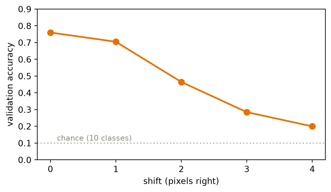
After the two-pixel shift, the accuracy falls from 76.0% to 46.5%.
Does the shift fail because it pushes garments off the canvas? Fashion-MNIST scales each garment’s longest edge to fill the frame (Xiao et al.), so wide items such as sandals, sneakers, and ankle boots reach the right border, and a two-pixel shift crops them. We measure the crop on its own by zeroing the same two columns without moving anything.
Measure how much ink the two cropped columns hold.
Zero those columns in place, leaving every garment where it was.
Print the two ink measurements and the validation accuracy with those columns zeroed.
# [1]edge = X_val.reshape(-1, 28, 28)[:, :, -2:] # the columns a 2px shift cropstouched = (edge.flatten(1) >0).any(dim=1).float().mean().item()ink_share = (edge.sum() / X_val.sum()).item()# [2]cropped = X_val.reshape(-1, 28, 28).clone()cropped[:, :, -2:] =0# [3]print(f"images with ink in the two cropped columns: {touched:.1%}")print(f"share of all ink in those columns: {ink_share:.1%}")print(f"columns zeroed in place, nothing moved: validation accuracy "f"{accuracy(net, cropped.reshape(-1, 784), y_val):.1%}")
images with ink in the two cropped columns: 35.0%
share of all ink in those columns:          1.2%
columns zeroed in place, nothing moved:     validation accuracy 74.0%
Removing those columns in place costs two percentage points, far less than the full shift. The crop-only control therefore does not account for the much larger loss after displacement.
This is the distinction from Chapter 1: validation data drawn from the data-generating distribution \(P\) estimates performance under \(P\), not automatically under a transformed distribution. If \(T\) shifts an image while preserving its label, then
where \(T_\#P\) is the distribution obtained by transforming inputs drawn from \(P\) while retaining their labels. The MLP generalized moderately from its fitting sample to fresh clean examples from \(P\), but it was not robust under \(T_\#P\). There is no contradiction. Clean validation and shift robustness answer different questions. We trained the model on clean images, then asked it to recognize shifted ones. The loss did not require robustness to that shift. Appendix E gathers the \(P\), \(T_\#P\), and deployment-distribution notation in one place.
As the validation images move right by 0 to 4 pixels, Figure 6.1 follows the same fixed network. We call the resulting drop in accuracy the shift cliff.
Measure validation accuracy at right shifts of 0 to 4 pixels and open the figure.
Plot accuracy vs. shift.
import matplotlib.pyplot as plt# [1]shifts =list(range(5))accs = [accuracy(net, shift_right(X_val, s), y_val) for s in shifts]plt.figure(figsize=(5.6, 3.3))# [2]plt.plot(shifts, accs, "o-", color="#E57200", lw=2, ms=7)plt.axhline(0.1, ls=":", color="#B8B8A8")plt.text(0.1, 0.115, "chance (10 classes)", color="#8A8A7A", fontsize=9)plt.xlabel("shift (pixels right)"); plt.ylabel("validation accuracy")plt.ylim(0, 0.9); plt.xticks(shifts)plt.tight_layout(); plt.show()
Figure 6.1: Validation accuracy of the clean-trained network under rightward shifts of the validation images. The network is not retrained, and the original labels are retained. The dotted line marks the ten-class chance level; accuracy approaches it by four pixels of shift.
Experiment 2: permute the pixel coordinates
We choose one fixed random permutation of the 784 pixel positions and apply it to every image, fitting and validation alike. We keep the original labels attached to the examples. The displayed arrays are no longer recognizable garments: the ordinary grid adjacency has been destroyed.
Unlike a small shift, this is not a transformation under which we require the clean-trained classifier to preserve its decision. A changed prediction after scrambling is not, by itself, a robustness failure. Nor does the scramble specify a different correct garment class. Instead, we ask a separate question: can a fresh model learn the original labels from this consistently re-encoded dataset? The permutation is invertible, so it changes where information is stored without removing it. Predict before retraining: does the altered arrangement cost this MLP five points, twenty, or almost nothing?
Set the seed to 0 and draw pixel_perm, a random reordering of the 784 pixel positions.
Retrain on one fixed permutation of the pixel coordinates.
Print validation accuracy for the original MLP and for the retrained MLP on shuffled images.
# [1]torch.manual_seed(0)pixel_perm = torch.randperm(784) # one fixed scrambling for all images# [2]net_shuffled = train_mlp(X_tr[:, pixel_perm], y_tr)# [3]print(f"original images: validation accuracy {accuracy(net, X_val, y_val):.1%}")print(f"shuffled pixels: validation accuracy "f"{accuracy(net_shuffled, X_val[:, pixel_perm], y_val):.1%}")
original images:  validation accuracy 76.0%
shuffled pixels:  validation accuracy 77.0%
The two validation accuracies are close in this one deterministic run. This is not an uncertainty estimate; it shows that the training recipe can learn a useful classifier in the scrambled representation.
The two experiments used different protocols. Experiment 1 kept the clean-trained model and changed only the validation images. Experiment 2 transformed both the fitting and validation images and retrained. Complete the other two cells of that two-by-two design:
Evaluate the clean model on scrambled images, without retraining.
Retrain the same MLP on shifted images, then evaluate it on shifted images.
Print validation accuracy for the scrambled, trained-clean case and the shifted, retrained case.
NoteDiagnostic protocol: a fixed model versus retraining
Validation accuracy for the four combinations of transformation and protocol; the clean-trained model scores 76.0% on untouched validation images. All scores use the original labels, including those attached to the scrambled inputs.
Protocol
Two-pixel shift
Fixed pixel scramble
Fixed model: trained clean, evaluated transformed
46.5%
8.0%
Retrained: trained and evaluated on transformed data
76.5%
77.0%
The two results in the first row have different interpretations. The shift result shows a failure of the desired tolerance to small position changes. The scramble result shows sensitivity to a much larger change in spatial organization, for which we did not require invariance. These are not two instances of the same robustness failure.
The second row shows that retraining recovers similar accuracy in both transformed datasets under this recipe. For the fixed scramble, the next section gives an exact coordinate-permutation argument. A zero-filled shift also discards boundary pixels, so its retrained result is empirical, not a consequence of that invertible symmetry.
Watch the mechanism: retrained scramble versus fixed-model shift
Retraining on one fixed scramble of the pixel positions reached an accuracy close to the original's; sliding the image two pixels under the clean model nearly halved its accuracy. Both rearrange the same pixels, but under different protocols. What does retraining change?
A single dense unit, drawn as the row of products it adds up: a schematic eight-pixel row in place of the chapter's 784, with the weights it was fitted against underneath.
The calculation is readable without playback. Opening this panel loads the optional controls.
This is one unit's arithmetic, not the chapter's experiment: nothing here is trained, no accuracy is measured, and the eight weights and pixel values are a declared schematic row standing in for 784.
Scope and caveats
The permutation is free only because it is applied to the weights as well, a parameterization that retraining on a scrambled world can reach; the two training runs correspond only in distribution, so a particular retrained run need not match the original's accuracy exactly. The chapter's protocol matrix fills in the other two cells: a permutation applied to the pixels of an already fitted model breaks the pairing exactly as a shift does, and retraining on shifted images recovers similar accuracy, an empirical result, since the zero-filled shift also discards boundary pixels. The asymmetry is between protocols, pixels and weights moved together versus pixels alone, not between scrambling and sliding; it is a statement about the hypothesis class, not about any particular fitted weight.
The slide follows the chapter's own shift_right: pixels move two places right, zeros enter at the left, and what runs off the right is lost. In a real image the slide is two-dimensional and a row of 784 wraps as 28 rows of 28, so a two-pixel horizontal shift moves each pixel two positions within its row rather than two positions along the flat vector; the one-dimensional row here keeps the re-pairing visible and drops that detail.
Nothing here explains how much accuracy either change costs. The chapter measures that, and the loss from a shift depends on what the fitted weights were doing, which no schematic row can say. Blue is the pixel input, orange the learnable weights, green the score they produce, and grey the reference the comparison beat keeps.
Check yourself. Take the fitted model and permute only the validation pixels, leaving the weights as they were. Would that cost accuracy — and does a convolutional layer share the dense layer's indifference to a common permutation?
Yes, and no. Permuting the pixels alone re-pairs every term exactly as a shift does, so the score changes and the accuracy collapses; the shuffle experiment recovers its accuracy only because it retrains. A convolution is not permutation-indifferent at all: its weights are tied to relative positions, so scrambling the grid destroys the adjacency it is built to exploit.
Transcript and keyboard help
Predict. Eight pixel values, 0.20, 0.90, 0.10, 0.60, 0.80, 0.30, 0.70 and 0.40, sit above the eight weights 0.90, minus 0.40, 0.20, 0.70, minus 0.60, 0.30, 0.80 and minus 0.10. No products are drawn yet.
The sum. Each weight multiplies the pixel above it: 0.18, minus 0.36, 0.02, 0.42, minus 0.48, 0.09, 0.56 and minus 0.04. Their total, the unit's score, is 0.39.
Hold. The pixel positions are about to be scrambled by one fixed permutation, and the model retrained, which can scramble the weights the same way. Predict the score before releasing it.
Scrambled together. Every column slides to a new place carrying both its pixel and its weight, so every product travels without changing height. The same eight numbers are added in a different order, and the score is 0.39 again.
Hold. The columns return to their original order, and now the pixels alone will slide two places to the right while the weights stay put, as when the clean model meets shifted images without retraining. Predict again.
Slid. The pixels move right by two, two zeros enter at the left, and the last two values fall off the end. Every weight now meets a different pixel, so the products are remade: 0.00, 0.00, 0.04, 0.63, minus 0.06, 0.18, 0.64 and minus 0.03. The score is 1.40.
Compare. A grey mark holds the score the unit had in place, 0.39, against the 1.40 the same weights now produce. The bar is three and a half times as long.
The lesson. A sum does not care what order its terms arrive in, which is why a permutation applied to both rows, as retraining allows, is free. It cares very much which weight met which pixel, which is why moving the pixels alone is not free, whether they slide or scramble.
Silent; paused initially; 1.5× playback. Focus the animation pane: Space or K plays/pauses, arrows seek between beats, Home/End jump, Escape pauses. The scrubber and speed menu also work by keyboard. Reduced-motion mode holds each beat's finished state instead of moving between them.
6.3 Inside the weights: full-frame templates
The distinction between a fitted model and its model family is explicit in the first layer. Write the fixed scramble as a permutation matrix \(\matr{P}\), so a scrambled image is \(\matr{P}\vect{x}\). For any first-layer matrix \(\matr{W}_1\), set \(\matr{W}_1' = \matr{W}_1\matr{P}^\top\). Then
because \(\matr{P}^\top\matr{P} = \matr{I}\). With the bias and later layers unchanged, the entire network produces the same output. Every function this MLP can compute in the original coordinates has a corresponding parameterization in the scrambled coordinates.
This is a property of the model family, not invariance of one fitted model. The equation changes the first-layer weights along with the inputs; keeping the weights fixed does not give the same identity. The initialization is exchangeable across input coordinates, and Adam applies the same coordinate-wise rule, so the training procedures correspond in distribution under a fixed permutation (Exercise 1). Resetting the seed does not itself permute the initial weights, so the two particular runs need not have identical accuracies.
The dense parameterization therefore gives no built-in preference to the original pixel adjacency over another ordering. It can still learn spatial regularities from data; it does not impose locality or translation invariance.
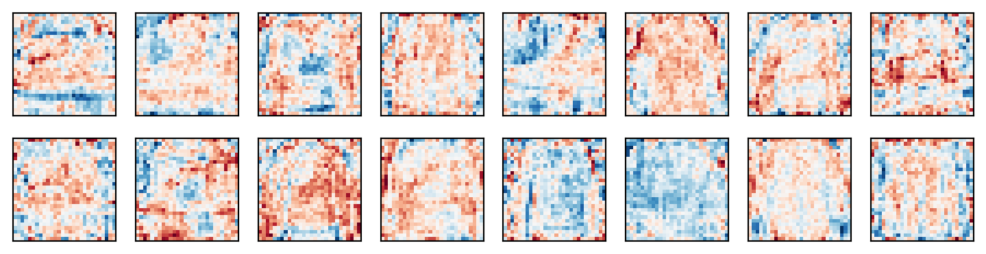
We can inspect that parameterization directly. Each row \(\vect{w}_j^\top\) of \(\matr{W}_1\in\mathbb{R}^{256\times784}\) assigns a separate coefficient to every input pixel. As in Chapter 1, it is a template scored by the inner product \(\langle\vect{w}_j,\vect{x}\rangle\). Reshaping the row into a 28×28 image shows its coordinate weights.
Figure 6.2: Sixteen first-layer weight rows with the largest norms, reshaped into images. The labeled scale runs from negative weights at the blue end through pale zero to positive weights at the red end. Each map shows a separate coefficient for every input pixel; its appearance alone does not establish what the full network recognizes or how robustly it does so.
We should not expect these maps to resolve into edges, contours, or parts that a person would name, and reading them is subjective. A picture of the weights cannot tell us whether the network will tolerate a spatial change or fail under it; only a transformation test can. What the maps do display is the full-frame parameterization: each hidden unit scores the image with an unconstrained template that spans the whole canvas, with an independent coefficient at every pixel coordinate. The layer contains no compact local detector that is reused at other positions.
For the pre-activation \(z_j(\vect{x})=\vect{w}_j^\top\vect{x}+b_j\), a transformation \(T\) changes the score by
The transformations of interest are label-preserving: small shifts of the garment within the frame, or a symmetry such as the left–right reflection of a shirt, after which the garment remains recognizable and its class is unchanged. A shift moves each intensity to a neighboring coordinate, where it is multiplied by a different coefficient, one that the dense parameterization leaves free of any tie to the first; only training decides how similar the two are. For a shift of \(s\) columns to the right, the ink in the \(s\) rightmost columns leaves the frame and changes the score as zeroing those columns in place would, the crop that Experiment 1 measured on its own. Every other pixel \(p\) moves to the position \(p+s\), \(s\) columns to its right, and these pixels contribute the rest of the difference, \(\sum_p (w_{j,p+s}-w_{j,p})\,x_p\), with the sum taken over them. The score change is therefore set by how each coefficient compares with its neighbor \(s\) columns away, a relation the dense layer leaves untied.
Asking each unit’s score to stay fixed would be the wrong remedy: for \(s=1\) it would force a template that is constant along every row and blind to horizontal arrangement. What the dense layer lacks is a unit tied to the shifted copy of \(\vect{w}_j\), so that the response could move with the garment, as the response of a shared local detector does. A change in one hidden score does not by itself settle the classifier’s decision either: the ReLU and the output layer combine all 256 hidden scores, whose changes can cancel or accumulate. Tolerance must therefore be measured at the output, as in Experiment 1.
During training, the gradient for row \(j\) is a weighted sum of the input images, \(\sum_i\delta_{ij}\,\vect{x}_i\), from the batched form of Equation 5.4. Adam rescales the coordinates separately, but neither that update nor the parameterization enforces a compact template or shared coefficients across positions. Expressive power alone does not supply the particular invariances we want. We next examine how clean performance changes with capacity.
6.4 Diagnosing the failure: capacity versus geometry
Is the model too flexible, or is the data too sparse for 784 dimensions?
Capacity: testing the classical U-curve
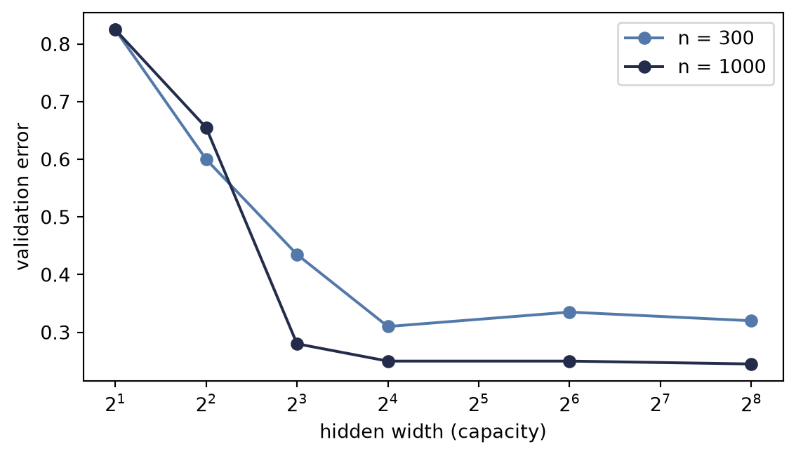
The classical picture, the cartoon of Chapter 1, predicts that as capacity grows, validation error first falls and then rises as the model overfits. A width sweep at two dataset sizes tests that prediction on real data:
Choose the hidden widths to sweep, from 2 up to 256 units.
Measure validation error across widths and fitting-set sizes.
# [1]widths = [2, 4, 8, 16, 64, 256]# [2]width_errors = { n: [1- accuracy(train_mlp(X_tr[:n], y_tr[:n], hidden=h, epochs=60), X_val, y_val)for h in widths]for n in (300, 1000)}
Figure 6.3: Testing the classical U-curve: validation error vs. hidden width at two fitting-set sizes. Error falls steeply as capacity grows, then flattens. In this one seeded sweep, n=300 shows a small late upturn while n=1000 does not.
The left side of the cartoon appears in both curves: networks with too little capacity underfit badly. The right side barely appears: a slight upturn at \(n = 300\) and a flat plateau at \(n = 1000\). The classical picture predicts a sustained rise in validation error once the width passes its best value; neither curve shows one. The U is a useful cartoon, not a law of nature (Chapter 1): the optimizer, the sample size, and the structure of the data can all shape the curve. A single seeded Adam sweep describes its own regime, so it cannot separate their effects, estimate a scaling law, or establish a \(1/n\) variance law.
The sweep measures clean validation performance, not shift robustness. It does not show that a smaller network would repair the baseline’s sensitivity to position: capacity and the response to a transformation require separate measurements.
Geometry: the curse of dimensionality
The width sweep leaves the shift failure unexplained, so we turn from the model to the representation it receives. How informative is distance between raw pixel vectors? Our images use 784 numbers; a small color image (32×32×3) uses 3,072, a one-megapixel color photo three million, and a 224×224×3 input 150,528. Covering every combination of pixel values is out of reach: a grid with 9 values per coordinate contains \(9^2\) points in two dimensions and \(9^d\) in \(d\) dimensions.
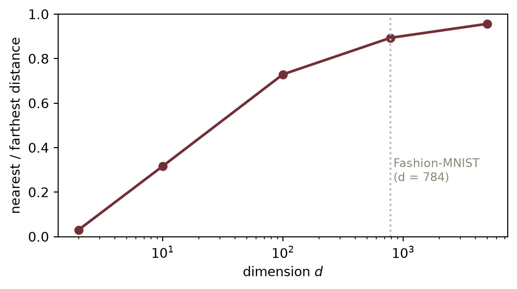
High dimension also erodes the contrast between near and far points:
Fix the seed, list dimensions from 2 to 5000, and start an empty ratios list.
Measure the nearest-to-farthest distance ratio by dimension.
# [1]torch.manual_seed(6050)dims = [2, 10, 100, 784, 5000]ratios = []# [2]for d in dims: P = torch.rand(300, d) D = torch.cdist(P, P) ratios.append(((D + torch.eye(300) *1e9).min(1).values / D.max(1).values).mean())
Figure 6.4: Distance concentration for 300 points sampled uniformly from a unit cube: the average ratio of nearest-neighbor to farthest-neighbor distance, by ambient dimension. At d=784 the ratio reaches 0.89. This is a controlled geometry example, not a claim that natural images fill the 784-dimensional cube uniformly.
Watch the mechanism: where "nearest neighbour" stops meaning anything
Covering 784 dimensions densely would take 9784 examples, so that route is closed. Then use the examples you have and trust the nearest ones — how near is the nearest, next to the farthest?
Not the chapter's measured curve but the geometry under it: the whole band of distances between two random points in a cube, drawn against the typical distance, as the dimension grows.
Width falls as one over the square root of d. Data cannot buy it back.
0:00 / 0:40
The calculation is readable without playback. Opening this panel loads the optional controls.
This is the unconstrained cube, not natural images: the chapter says so plainly, and structured data may concentrate near a much lower-dimensional set where near neighbours still exist.
Scope and caveats
The band is a closed-form estimate, not a simulation. For two points drawn uniformly from the unit cube the squared distance has mean d/6 and variance 7d/180, so the distance itself has a standard deviation that tends to a constant while its mean grows like the square root of d: the relative spread is the square root of 0.35 divided by d. The band's edges are placed at the expected extreme of a sample that size, which for 300 points is about 2.7131 standard deviations either way. Nothing here is sampled and no seed is used, so the panel's numbers are not the chapter's run — they are what its run should find, and at 784 dimensions they agree to the printed digit.
The ladder starts at ten dimensions because the estimate is a large-d one: at the chapter's smallest dimension, two, the spread is so large that the band would reach below zero, which is a sign the normal approximation has stopped applying rather than a claim about distance. The chapter's own measurement covers that case.
The ratio drawn here is the ratio of the extremes of the whole band, which is the same quantity the chapter averages over points, not a per-point average; the two agree at 784 to the digit the chapter prints. Grey is the band and the scenery, and the book's ink marks the two extremes and the ratio they make.
Check yourself. A dataset lives in 784 dimensions but every example actually lies on a smooth 12-dimensional surface inside it. Which number governs whether near neighbours still mean something — and by roughly how much does the band widen?
The intrinsic 12, not the ambient 784. The spread goes as one over the square root of the dimension that the data actually varies in, so the band is about eight times wider than the ambient number suggests — the square root of 784 over 12. That is why representation learning is worth so much: it is the dimension you cannot see that sets the price.
Transcript and keyboard help
Predict. An axis measuring distance against the typical distance between two random points in a cube. Nothing is drawn on it yet.
Ten dimensions. The band of distances runs from 0.49 to 1.51 times typical: the nearest point is a third as far as the farthest, a ratio of 0.33. Near still means something.
A hundred. The band has narrowed to 0.84 and 1.16, and the ratio has climbed to 0.72. The nearest point is already nearly as far away as the farthest.
Hold. Fashion-MNIST lives in 784 dimensions. Predict the ratio there before releasing it.
Seven hundred and eighty-four. The band spans 0.94 to 1.06 and the ratio is 0.89 — the number the chapter measures with 300 sampled points, recovered here from geometry alone.
Five thousand. The band is a sliver, 0.98 to 1.02, and the ratio is 0.96. Every point is the same distance from every other.
Compare. The band from ten dimensions returns as a dashed outline behind the sliver: the collapse is a shape against a shape, not two numbers.
The law. The band's width falls as one over the square root of the dimension, so closing it by a factor of ten costs a hundredfold in dimension, and no amount of data reopens it.
Silent; paused initially; 1.5× playback. Focus the animation pane: Space or K plays/pauses, arrows seek between beats, Home/End jump, Escape pauses. The scrubber and speed menu also work by keyboard. Reduced-motion mode holds each beat's finished state instead of moving between them.
In the uniform cube, nearest and farthest distances draw together as the dimension grows. Natural images are structured and may concentrate near a much lower-dimensional set, so this is not their empirical distance distribution. Nor is the \(9^d\) grid count a bound on the data needed for translation tolerance: a translation is described by two numbers, a horizontal and a vertical offset, not by independent changes to every pixel.
We now measure the pixel geometry of the actual images. How far does a two-pixel shift carry an image, compared with its distance to the nearest fitting image?
Measure how far the shift moves each validation image, and how far its nearest training image is.
Print the share of validation images where moved exceeds nearest, and both median distances.
# [1]moved = (X_val - shift_right(X_val, 2)).norm(dim=1) # (200,)nearest = torch.cdist(X_val, X_tr).min(dim=1).values # (200,)# [2]print(f"shift moves farther than the nearest training image: "f"{(moved > nearest).float().mean().item():.1%} of validation images")print(f"median distances: shifted copy {moved.median().item():.2f}, "f"nearest training image {nearest.median().item():.2f}")
shift moves farther than the nearest training image: 91.0% of validation images
median distances: shifted copy 7.78, nearest training image 4.55
In raw pixel space, then, a label-preserving shift can carry an image farther from the original than the nearest fitting image is. This diagnoses a mismatch between Euclidean pixel distance and the tolerance the task requires; it does not show that more data or augmentation cannot improve robustness. We next consider how to build the relevant structure into training and into the architecture.
6.5 Inductive bias: constraints as knowledge
Recall inductive bias from Chapter 1: the assumptions and preferences that distinguish fitted solutions beyond their agreement with the training sample. Here we have prior knowledge about image structure and about which position changes should preserve the label. Two principles suggest how to use it:
Locality. Nearby pixels jointly form edges, textures, and parts. Local connectivity gives these relationships a structural role that the dense parameterization does not assign them.
Translation structure. A local detector’s response should move with the feature (equivariance), while a classifier’s final prediction should tolerate or ignore small changes in position (invariance). The shift experiment tests this desired tolerance at the classifier’s output.
Data augmentation: specifying label-preserving transformations
The shift cliff suggests another route. If moving a garment a little should not change its class, let \(T\) be a random label-preserving transformation drawn from a declared distribution \(\mathcal{A}\). The population objective becomes
This is data augmentation, and its role is larger than making the dataset look bigger. It is a data-side inductive bias: the transformation distribution states which changes we believe should preserve the target. Sampling shifts from \(-3\) to \(+3\) pixels says that location within that window is a nuisance. This is an assumption about the task: complete pixel scrambling is not included in that invariance requirement. Retraining on one fixed scramble instead changes the encoding of the whole dataset. The empirical augmented objective used in training replaces the outer expectation with the sample average. Drawing one fresh \(T\) when an example enters a batch then gives a Monte Carlo estimate of the inner expectation. Exercise 2 asks you to include those shifts in the training batches and measure both what the augmentation buys on the shift curve and what it costs on clean images. Appendix E summarizes the corresponding estimators and distributions.
Augmentation encourages translation tolerance by training on shifted examples. It does not tie parameters across positions: a dense network still assigns them separate coefficients. Weight sharing imposes that relation directly. Exercise 2 measures the effect of augmentation with the current MLP; Part II develops the architectural alternative.
We can now place three familiar levers side by side:
Architecture-side bias changes which functions are available or easy to learn. Local connectivity and shared convolutional filters are the route Part II will take.
Objective- or training-side bias changes which fitted solution is preferred. Weight penalties, dropout, and early stopping from Chapter 4 are examples; the minibatch noise discussed there may also bias which solution training reaches.
Data-side bias changes the examples the model is fitted to. Augmentation encodes a chosen family of label-preserving transformations.
These routes can work together, but they are not interchangeable. A finite set of augmented shifts encourages consistency; it does not prove exact invariance. An architectural constraint can make a symmetry exact in a layer, but may exclude useful functions. A penalty prefers some solutions without specifying which input changes should preserve a label. And augmentation needs a label-preserving transformation: flipping a garment may be harmless, while flipping a digit or a directional sign may change the answer.
For Part II we begin with the architecture-side move: build locality and translation structure into the network itself as constraints. Constrain each template to look at a small local patch instead of the whole frame. Then share that template across every position, so the local detection rule uses the same parameters throughout the image. These constraints supply locality and sharing; the full classifier’s shift tolerance will still need to be evaluated. The parameter count falls too: our MLP has 203,530 parameters, while the LeNet model in Chapter 9 will have 61,706, less than a third as many.
TipWhy a constraint can add knowledge
Local connectivity and weight sharing constrain a corresponding dense network with the same layer sizes. Through Chapter 1’s bias–variance lens, we accept assumptions about image structure to reduce the space of solutions considered. When those assumptions are appropriate, the restriction can improve data efficiency. The choice remains task-dependent: we want tolerance to small position changes, not indifference to arbitrary rearrangements of the pixels. With sufficient data and a suitable training recipe, architectures with weaker spatial constraints can also perform well, as Vision Transformers illustrate in Chapter 19.
6.6 Toward local, shared detectors
The dense templates of Figure 6.2 assign separate coefficients across the whole image. Our next model will instead use small, local templates and apply the same weights at each position. Learning a local detection rule will then determine how that rule is applied elsewhere in the image.
Sliding a local template across the image and scoring each position by an inner product is a classical operation, decades older than deep learning. Part II opens by building this operation by hand and then poses the following question:
What if the template were learnable?
6.7 One sealed test check
We have now fixed the architecture, optimizer, shift size, and reported metrics. Only now do we fit the same MLP on all 1,200 development examples and open the 600-example test set once:
Run one final test-set check.
Print the final model’s test accuracy on clean and two-pixel-shifted images.
# [1]net_final = train_mlp(X_dev, y_dev)# [2]print(f"clean test accuracy: {accuracy(net_final, X_test, y_test):.1%}")print(f"shift-2 test accuracy: "f"{accuracy(net_final, shift_right(X_test, 2), y_test):.1%}")
clean test accuracy:   80.8%
shift-2 test accuracy: 42.0%
The sealed check confirms the diagnostic rather than creating it: 80.8% on clean test images becomes 42.0% after the predeclared two-pixel shift.
NoteCheck yourself
Close the book for one minute and test the argument on these three questions.
Why do we require tolerance to a small shift but not to complete pixel scrambling? What separate question does retraining on a fixed scramble answer?
Where can inductive bias enter: architecture, objective, or data? Give one example of each.
Why can high clean validation accuracy coexist with collapse after a two-pixel shift?
6.8 Okay, so: the missing ingredient is inductive bias
Clean accuracy and shift robustness are different claims. The MLP predicts well on clean held-out images but loses accuracy after a small, label-preserving displacement.
Invariance must match the task. A complete scramble changes the spatial organization and need not preserve a clean-trained model’s decision. Retraining on that fixed permutation tests learning in a different encoding, not invariance of the original classifier.
The model family has a coordinate symmetry. The reparameterization in Equation 6.2 explains why a dense architecture gives no built-in preference to the original pixel ordering. The weight maps display its coordinate-specific coefficients; appearance alone does not establish robustness or its cause.
Capacity and ambient dimension do not settle the diagnosis. The width sweep describes one clean-data regime, and the uniform-cube example illustrates distance concentration under its own distribution. Neither gives a general limit on what structured data or augmentation can achieve.
Inductive bias specifies useful structure. It can enter through architecture, objectives, training procedures, or data. Part II develops locality and weight sharing; augmentation is a complementary way to specify which transformations should preserve the label.
Deeper dive
NoteFor the curious: memorization, confidence, and double descent
Networks can memorize random labels. Zhang et al. reported 100% training accuracy on randomly labeled CIFAR-10 and 95.20% on randomly labeled ImageNet under their finite training budget, not 100% on ImageNet. Capacity is abundant enough that fitting noise is easy (Exercise 4 reproduces the phenomenon on our subset). Capacity alone therefore does not explain generalization; the data, optimizer, and architecture must enter the account.
Confident far from the data. A trained ReLU network is piecewise affine: its input space splits into polyhedral regions, and on each one the logits \(o_k=\vect{w}_k^\top\vect{x}+b_k\) are affine in \(\vect{x}\). Along a ray that remains in one such region, if one logit has a strictly larger slope than the others, its softmax probability approaches 1 as the distance increases. Hein, Andriushchenko, and Bitterwolf analyze this behavior for ReLU classifiers. High softmax confidence therefore need not indicate that an input resembles the training data. This is a separate question from the label-preserving shift test.
The bias–variance picture, updated. Test error can sometimes descend again beyond the interpolation threshold, where the model first becomes able to fit the training sample exactly: “double descent.” The width sweep above does not establish that pattern. It illustrates why a classical U-shaped curve should not be assumed in every training regime.
Grant Sanderson, Analyzing Our Neural Network (3Blue1Brown, 2017; text adaptation by Josh Pullen): a related visual examination of first-layer weights and the limits of a trained digit classifier. The transformation comparisons here use the Fashion-MNIST model and protocols specified in this chapter.
(Pencil.)Equation 6.2 handles a fixed permutation. (a) Write the zero-fill two-pixel shift as a \(784\times784\) matrix \(\matr{S}\) and show that it is a partial permutation: which rows are zero, and why, for a general \(\matr{W}_1\), can no \(\matr{W}_1'\) satisfy \(\matr{W}_1'\matr{S}\vect{x} = \matr{W}_1\vect{x}\) for every image? (b) Argue that if the initialization is exchangeable across input coordinates and the optimizer treats coordinates alike, training on \(\matr{P}\vect{x}\) produces, in distribution, the weights \(\matr{W}_1\matr{P}^\top\). With the same seed, the scrambled run scores 77.0% and the original run 76.0%. Which random choices do the two runs share, and which of them do not correspond under the permutation?
(Code.) Augment the training set with random shifts of ±3 pixels and retrain. Re-plot the cliff. How much shift robustness did augmentation buy, what did it cost in clean accuracy and compute, and what data-side inductive bias did augmentation encode, compared with imposing locality and weight sharing in the architecture?
(Code.) The width sweep used widths up to 256. Push to 1024 and 4096 at \(n = 300\), repeating each width across several seeds. Then compare Adam with minibatch SGD from Chapter 4. Which patterns are stable enough to interpret?
(Code.) Random-label audit. (a) Randomly permute the training labels and train a wide MLP for long enough. Report train and test accuracy. (Audit.) (b) Use Table 6.1 to state what successful fitting supports. Explain why one successful run proves neither that the objective is convex, nor that bad local minima are absent, nor that the fitted rule will generalize.
(Pencil.) Estimate the first-layer parameter count of an MLP with 1,000 hidden units on an ImageNet-scale input (224×224×3). At one float32 per parameter, how much memory is that, and how does the number change if each unit instead sees only a 7×7×3 patch?
(Pencil.) Count the labelings of \(N\) ordered points realizable by (a) positive rays on a line, (b) intervals on a line, and (c) affine linear separators for \(N\) points in general position in two dimensions. Obtain \(N+1\), \(N(N+1)/2+1\), and \(2\sum_{i=0}^{2}\binom{N-1}{i}\), respectively. Compare each with \(2^N\). Do not invoke VC dimension: the point is to see, with arithmetic, how restricting the hypothesis menu changes its growth.