15  Attention: Making the Kernel Learnable

Chapter tools Lecture 8.1 · Attention Mechanism I·Lecture 8.2 · Attention Mechanism II·Lecture 8.3 · Adding Attention to a Seq2Seq Decoder·Download notebook·Open in Colab (opens in a new tab)

Chapter 14 built the whole attention operator except for one piece. It had a query, a bank of keys and values, a score for every query–key pair, softmax weights, and a weighted read. But Euclidean distance decided what counted as similar. The task could tune the bandwidth; it could not invent a better notion of relevance.

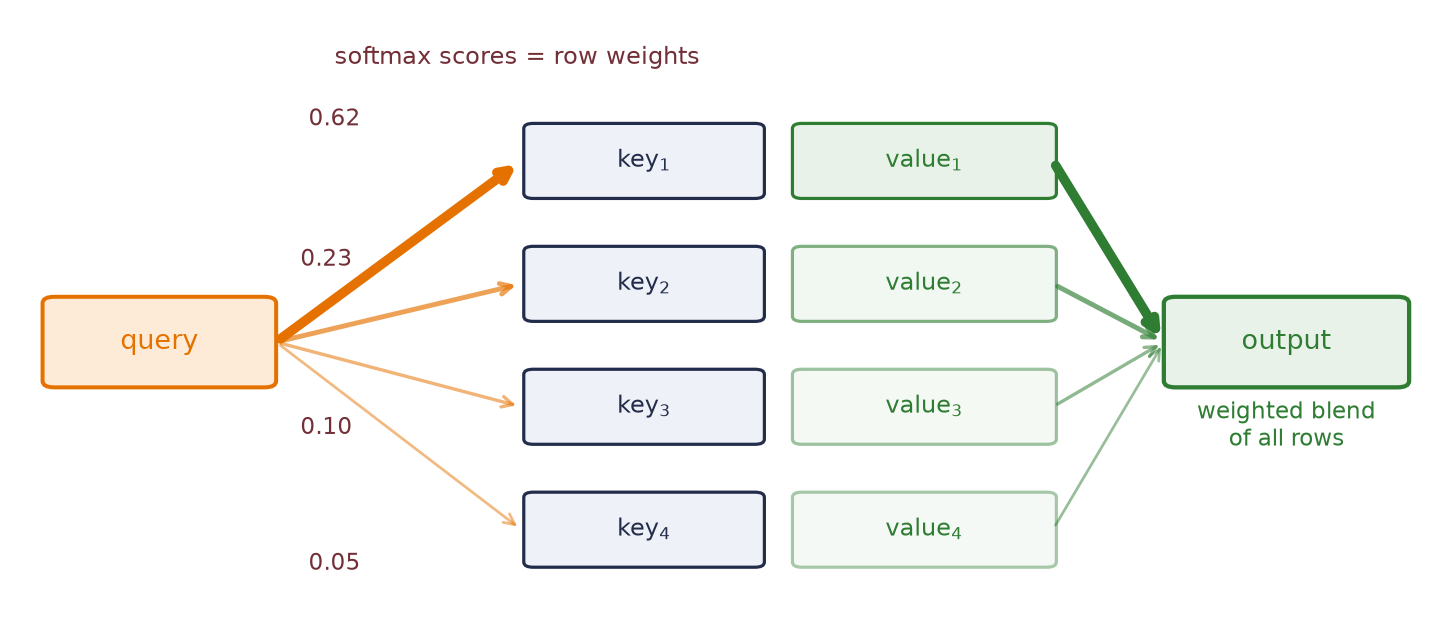
An embedding can learn what lives at row 17, but fetching row 17 is still a rigid act of indexing: learned content behind a hard address. Replace the one address with a distribution over addresses, let the gradient reach every score, and the model can learn which rows deserve weight. Compare one request with every stored candidate, normalize the scores with Chapter 2’s softmax, and blend the stored values with the resulting weights. This content-dependent weighted read is attention.

Figure 15.1: The lookup table, softened. A hard lookup would follow exactly one arrow to one row. Attention scores the query against every key, softmax turns the scores into row weights (arrow thickness; the numbers here are illustrative), and the output is the weighted blend of all values. Every arrow is differentiable, so the loss can teach the scoring itself.

The result is visible in the date task before we name all its parts. For the fixed validation source

may 17, 1971  ->  1971-05-17

the trained decoder emits the year first even though those four characters sit at the end of the source. Across the fixed 400-example validation audit, its first four attention rows place 97.5% of their mass on the four contextual encoder states indexed by the source-year characters. When the example above emits its second character, 9, the largest weight is 0.856 on the state indexed by the source’s 9; when it emits 7, the largest weight is 0.985 on the state indexed by the 7 in the year region. Those weights were not supervised as alignments. The date loss taught the model where useful information lived.

15.1 The scores-to-weights machine, one more time

Let the encoder retain its full memory

\[ \matr{H}=[\vect{h}_1,\ldots,\vect{h}_n]^\top \in\mathbb{R}^{n\times d_e}. \]

At decoder step \(t\), use the previous decoder hidden state \(\vect{s}_{t-1}\in\mathbb{R}^{d_d}\) as the query. A learned compatibility function \(a_\theta\) produces one score per source position:

\[ e_{t,i}=a_\theta(\vect{s}_{t-1},\vect{h}_i). \]

For each padded batch item \(b\), let \(M_{b,i}=0\) at real source positions and \(M_{b,i}=-\infty\) at padding. Suppress the batch index below. Then

\[ \alpha_{t,i} =\operatorname{softmax}_i(e_{t,i}+M_i), \qquad \vect{c}_t=\sum_{i=1}^{n}\alpha_{t,i}\vect{h}_i. \tag{15.1}\]

This is Chapter 14’s fixed matrix \(\matr{A}\matr{V}\) with a learned score. The softmax is unchanged; we now learn the scoring rule. A hard source-position choice would use argmax and one-hot indexing. The soft weights move continuously when the scores move, so backpropagation can tell the scorer how each valid address affected the loss. We have softened the hard.

Because the query comes from the decoder and the memory comes from the encoder, this is cross-attention. It bridges two sequences. The model still initializes the decoder from the encoder’s final state, but that fixed bridge is no longer the only path from source to output: every decoder step receives its own context \(\vect{c}_t\). The old handoff was a finite-state bottleneck. Chapter 14 kept the memory bank; cross-attention now learns the rule that reads it.

In Chapter 9, a CNN saw the whole input only by stacking local operations until its receptive field spanned it. One cross-attention read can score every encoder position in a single layer. It reaches the whole input directly, at the cost of every query–key comparison. For now, the encoder states it reads still come from RNNs that compute them one step at a time.

15.2 Additive attention: learn the comparison itself

The most literal answer to “make similarity learnable” is a small neural network. Choose an alignment width \(d_a\). For one decoder query and one encoder state,

\[ e_{t,i} =\vect{v}_a^\top \tanh\!\left( \matr{W}_q\vect{s}_{t-1} +\matr{W}_k\vect{h}_i \right), \tag{15.2}\]

where

\[ \matr{W}_q\in\mathbb{R}^{d_a\times d_d}, \qquad \matr{W}_k\in\mathbb{R}^{d_a\times d_e}, \qquad \vect{v}_a\in\mathbb{R}^{d_a}. \]

The two projections put objects of different native sizes into one alignment space. The tanh creates match features, and \(\vect{v}_a\) selects which of those features matter for the scalar score. The same parameters are reused for every decoder step \(t\) and source position \(i\). Remember Chapter 9’s sliding filter, which applied one learned rule everywhere. Attention shares a compatibility rule across pairs.

For a batch, let \(\matr{S}_{t-1}\in\mathbb{R}^{B\times1\times d_d}\) collect the queries. The row-major shapes make the broadcasting explicit:

\[ \matr{S}_{t-1}\matr{W}_q^\top: (B,1,d_a), \qquad \matr{H}\matr{W}_k^\top: (B,n,d_a). \]

Their sum produces \((B,n,d_a)\) match features. Reduction by \(\vect{v}_a\) produces \((B,n)\) scores, softmax runs over the \(n\) source positions, and the weighted read returns a \((B,d_e)\) context. Softmax over the wrong dimension would answer the wrong question.

We freeze one simple parameter snapshot so we can watch the arithmetic. With identity projections and an all-ones selector, three source states receive scores \((1.015,1.562,1.124)\) and therefore weights \((0.260,0.450,0.290)\):

1. Compute the three-key additive scores and softmax weights.

from __future__ import annotations

import math
import random

import matplotlib.pyplot as plt
from matplotlib.patches import FancyBboxPatch
import numpy as np
import torch
import torch.nn as nn
import torch.nn.functional as F
torch.set_num_threads(4)  # pinned: results depend on the CPU thread count

# [1]
torch.manual_seed(6050)

query_snapshot = np.array([0.5, 0.5, 0.2, -0.1])
key_snapshot = np.array([
    [-0.3, 0.1, 0.2, 0.0],
    [0.6, 0.5, 0.1, -0.2],
    [0.0, -0.4, 0.3, 0.2],
])
snapshot_scores = np.tanh(query_snapshot + key_snapshot).sum(axis=1)
snapshot_weights = np.exp(snapshot_scores - snapshot_scores.max())
snapshot_weights /= snapshot_weights.sum()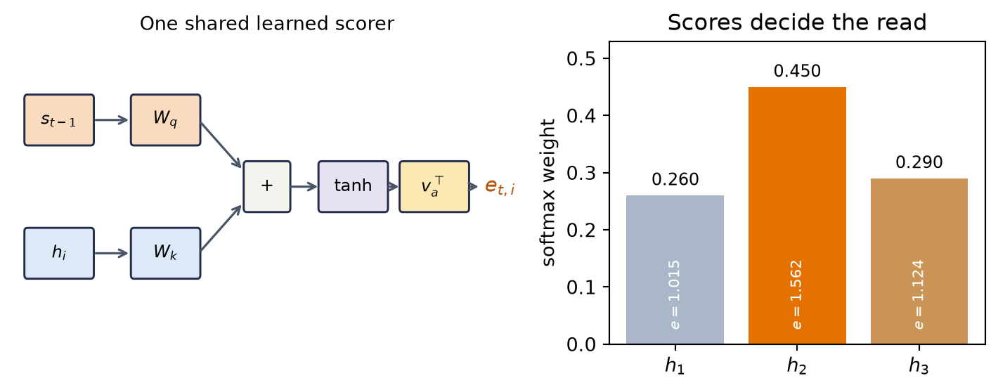

Figure 15.2: Additive attention learns a compatibility function. Query and key enter separate projections, their alignment features interact through tanh, and a learned selector reduces those features to one score. The right panel freezes one parameter setting to show the resulting scores-to-weights calculation; it is arithmetic, not a trained result.

Note“Learned kernel” is an analogy

Exponentiating a learned score and normalizing it reproduces the Nadaraya–Watson algebra. It does not make every attention score a classical kernel. Separate query and key projections can make \(a_\theta(q,k)\) asymmetric and not positive semidefinite. What survives exactly is the operational pattern: compare \(\rightarrow\) normalize \(\rightarrow\) mix.

15.3 Scaled dot product: learn the spaces, simplify the score

For \(m\) decoder queries, additive attention is vectorized, but it forms a \((B,m,n,d_a)\) intermediate, applies an elementwise tanh, and reduces it. Dense matrix multiplication has a simpler computational path. Chapter 1 introduced the dot product as a similarity score against a template. Here the key is the template, and training learns the space in which that comparison is useful.

First walk one four-dimensional query past three keys. Its raw dot products are \((1.10,-0.60,0.15)\). Since \(\sqrt{4}=2\), scaling gives \((0.55,-0.30,0.075)\), and softmax gives \((0.488,0.209,0.303)\):

1. Set a four-dimensional query and three keys, then compute raw_walk, scaled_walk, and weight_walk.
2. Run one query through dot product, scaling, and softmax.

# [1]
query_walk = torch.tensor([0.9, -0.3, 0.2, 0.6])
key_walk = torch.tensor([
    [0.8, -0.2, 0.1, 0.5],
    [-0.5, 0.9, 0.0, 0.2],
    [0.3, 0.0, 0.6, -0.4],
])
raw_walk = key_walk @ query_walk
scaled_walk = raw_walk / math.sqrt(query_walk.numel())
weight_walk = torch.softmax(scaled_walk, dim=0)
# [2]
print("raw scores:", raw_walk.numpy())
print("scaled scores:", scaled_walk.numpy())
print("weights:", weight_walk.numpy(), "sum:", weight_walk.sum().item())

raw scores: [ 1.0999999 -0.6        0.15     ]
scaled scores: [ 0.54999995 -0.3         0.075     ]
weights: [0.4879715  0.20856632 0.3034622 ] sum: 1.0

Now let raw decoder features \(\matr{D}\in\mathbb{R}^{B\times m\times d_d}\) and encoder memory \(\matr{H}\in\mathbb{R}^{B\times n\times d_e}\) enter learned projections:

\[ \begin{aligned} \matr{Q}&=\matr{D}\matr{W}_Q, &\matr{W}_Q&\in\mathbb{R}^{d_d\times d_k},\\ \matr{K}&=\matr{H}\matr{W}_K, &\matr{W}_K&\in\mathbb{R}^{d_e\times d_k},\\ \matr{V}&=\matr{H}\matr{W}_V, &\matr{W}_V&\in\mathbb{R}^{d_e\times d_v}. \end{aligned} \]

The resulting tensors have shapes

\[ \matr{Q}\in\mathbb{R}^{B\times m\times d_k},\qquad \matr{K}\in\mathbb{R}^{B\times n\times d_k},\qquad \matr{V}\in\mathbb{R}^{B\times n\times d_v}. \]

Only the projected query and key widths must agree. The raw encoder and decoder widths need not. Let \(\matr{M}\in\mathbb{R}^{B\times1\times n}\) broadcast across queries. Scaled dot-product attention is

\[ \operatorname{Attention}(\matr{Q},\matr{K},\matr{V}) =\operatorname{softmax}\!\left( \frac{\matr{Q}\matr{K}^{\top}}{\sqrt{d_k}}+\matr{M} \right)\matr{V}, \tag{15.3}\]

where \(\matr{K}^{\top}\) transposes the last two axes within each batch. Softmax runs over the last, key-position axis. The hot path is two dense products: \(\matr{Q}\matr{K}^{\top}\) and \(\matr{A}\matr{V}\). Additive attention remains useful and accelerator-compatible; scaled dot product maps more directly to the matrix operations modern numerical libraries optimize heavily.¹

Luong and colleagues compared unscaled dot, general, and concat scores in recurrent translation. Vaswani and colleagues later introduced the \(1/\sqrt{d_k}\) scaling in the Transformer formulation. The mechanisms belong in one conceptual family, not a single inevitable historical derivation.

The dot product is not magically semantic. \(\matr{W}_Q\) and \(\matr{W}_K\) learn which features to compare, including their magnitudes, while the surrounding RNN has already built nonlinear sequence features.²

Why divide by \(\sqrt{d_k}\)?

Suppose, for the moment, that projected coordinates \(q_\ell\) and \(k_\ell\) are independent, mean zero, and variance one, and that their products are independent across coordinates. Then

\[ \E[\vect{q}^{\top}\vect{k}]=0, \qquad \var(\vect{q}^{\top}\vect{k}) =\sum_{\ell=1}^{d_k}\var(q_\ell k_\ell)=d_k. \]

The score’s standard deviation grows as \(\sqrt{d_k}\). Dividing by that quantity returns the idealized variance to one. Trained projections need not stay independent or unit variance.

We test both the score variance and the average largest softmax weight. For each width, we draw 20,000 queries and 16 independent keys per query:

1. Create a seeded generator and an empty scaling_rows list for per-width results.
2. Audit score variance and softmax concentration versus width.
3. Print, for each width, the raw and scaled score variances and largest softmax weights.

# [1]
scaling_gen = torch.Generator().manual_seed(6050132)
scaling_rows = []
# [2]
for width in (8, 32, 128, 512):
    raw_parts, raw_max_parts, scaled_max_parts = [], [], []
    for _ in range(20_000 // 500):
        q = torch.randn(500, 1, width, generator=scaling_gen)
        k = torch.randn(500, 16, width, generator=scaling_gen)
        raw = (q * k).sum(-1)
        raw_parts.append(raw.reshape(-1))
        raw_max_parts.append(torch.softmax(raw, dim=-1).max(-1).values)
        scaled_max_parts.append(
            torch.softmax(raw / math.sqrt(width), dim=-1).max(-1).values
        )
    raw_scores = torch.cat(raw_parts)
    scaling_rows.append((
        width,
        raw_scores.var(unbiased=True).item(),
        (raw_scores / math.sqrt(width)).var(unbiased=True).item(),
        torch.cat(raw_max_parts).mean().item(),
        torch.cat(scaled_max_parts).mean().item(),
    ))

# [3]
print("d_k   raw var   scaled var   raw max-w   scaled max-w")
for row in scaling_rows:
    print(f"{row[0]:3d}   {row[1]:8.3f}   {row[2]:10.3f}   "
          f"{row[3]:9.3f}   {row[4]:12.3f}")

d_k   raw var   scaled var   raw max-w   scaled max-w
  8      8.023        1.003       0.564          0.241
 32     32.142        1.004       0.779          0.246
128    127.985        1.000       0.889          0.246
512    510.347        0.997       0.944          0.247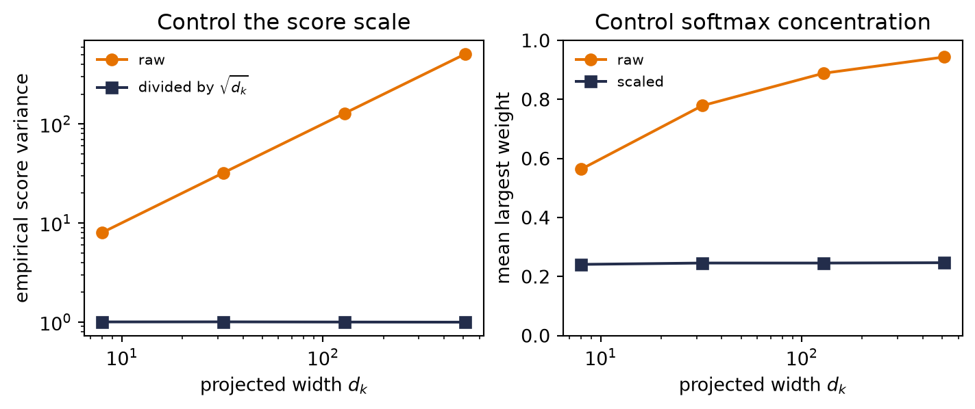

Figure 15.3: The scaling argument under its stated random-feature assumptions. Left: raw dot-product variance grows with width, while division by the square root of the width keeps it near one. Right: without scaling, a 16-key softmax becomes nearly one-hot as width grows; scaling keeps its mean largest weight near one quarter (0.24 in this draw). These are seeded synthetic draws about concentration, not a claim about every trained layer’s gradients.

Raw variance rises from \(8.02\) to \(510.35\) as \(d_k\) grows from 8 to 512. Scaled variance stays between \(0.997\) and \(1.004\). Over the same range, the average largest unscaled softmax weight climbs from \(0.564\) to \(0.944\); the scaled value stays between \(0.24\) and \(0.25\). This is Chapter 2’s temperature dial, set by the dimension. Scaling corrects the dimension-induced spread; it does not normalize the vectors.

15.4 Mask before softmax, and mask the right thing

Padding affects two computations, as Chapter 13 showed: the loss and an encoder’s final state. Attention creates a third place to enforce sequence lengths: the score matrix. A padded key must not receive a merely mediocre score. It must be excluded before normalization. Setting its score to zero is wrong because \(\exp(0)=1\) still earns weight.

The scaled-dot operator below accepts already projected queries, keys, and values, then audits a batch whose second example has two padded keys:

1. Define the reusable scaled_dot_attention helper.
2. Run and audit scaled dot-product attention with a source-padding mask.

# [1]
def scaled_dot_attention(
    queries: torch.Tensor,
    keys: torch.Tensor,
    values: torch.Tensor,
    key_is_valid: torch.Tensor,
) -> tuple[torch.Tensor, torch.Tensor]:
    """Attend with Q:(B,m,d_k), K:(B,n,d_k), V:(B,n,d_v)."""
    if queries.ndim != 3 or keys.ndim != 3 or values.ndim != 3:
        raise ValueError("Q, K, and V must be three-dimensional")
    if queries.shape[-1] != keys.shape[-1]:
        raise ValueError("projected Q and K widths must match")
    if keys.shape[:2] != values.shape[:2]:
        raise ValueError("K and V must have the same batch and key axes")
    if key_is_valid.shape != keys.shape[:2] or not key_is_valid.any(dim=1).all():
        raise ValueError("every example needs at least one valid key")

    scores = queries @ keys.transpose(-2, -1) / math.sqrt(keys.shape[-1])
    scores = scores.masked_fill(~key_is_valid[:, None, :], -torch.inf)
    weights = torch.softmax(scores, dim=-1)
    return weights @ values, weights

# [2]
mask_gen = torch.Generator().manual_seed(6050133)
Q_demo = torch.randn(2, 2, 4, generator=mask_gen)
K_demo = torch.randn(2, 4, 4, generator=mask_gen)
V_demo = torch.randn(2, 4, 3, generator=mask_gen)
valid_demo = torch.tensor([[True, True, True, True],
                           [True, True, False, False]])
context_demo, mask_weights = scaled_dot_attention(
    Q_demo, K_demo, V_demo, valid_demo
)
assert torch.allclose(
    mask_weights.sum(-1), torch.ones_like(mask_weights[..., 0])
)
assert torch.count_nonzero(mask_weights[1, :, 2:]) == 0
print("Q", tuple(Q_demo.shape), "K", tuple(K_demo.shape),
      "V", tuple(V_demo.shape), "A", tuple(mask_weights.shape),
      "AV", tuple(context_demo.shape))
print("maximum row-sum error:",
      f"{(mask_weights.sum(-1) - 1).abs().max().item():.2e}")
print("maximum padded weight:",
      f"{mask_weights[1, :, 2:].max().item():.1f}")

Q (2, 2, 4) K (2, 4, 4) V (2, 4, 3) A (2, 2, 4) AV (2, 2, 3)
maximum row-sum error: 0.00e+00
maximum padded weight: 0.0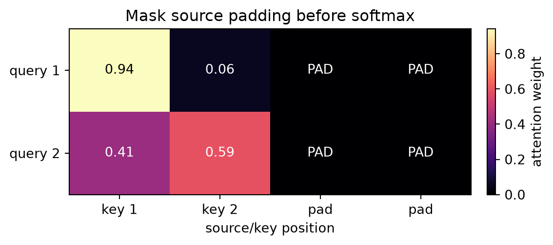

Figure 15.4: A source-padding mask acts before softmax. The second example has only two real keys; its last two score cells are excluded and receive exactly zero weight. Cross-attention may read every real source position, so no causal triangle belongs here.

Watch the mechanism: zero is not a padding mask

Does giving padding a score of zero exclude it?

Follow query 2 of the audit's second example. These are its existing four keys, with the intermediate scores made visible.

\( \class{mbs-probability}{\predictionpart{\alpha_j}}=\dfrac{\class{mbs-numerator}{\exp(s_j)}}{\class{mbs-denominator}{\sum_k\exp(s_k)}} \) \( \class{mbs-zero}{\exp(0)=1} \) \( \class{mbs-exclude}{\exp(-\infty)=0} \)

Keep at least one real key. An all-masked row has no distribution to normalize.

The calculation is readable without playback. Opening this panel loads the optional controls.

This expands the existing seeded audit, not a new sample or a trained alignment.

Scope and caveats

The formula uses the scores currently shown. Setting padded scores to zero is deliberately wrong; negative infinity excludes them before normalization. This is source-padding masking, not target-loss or causal masking: all real source keys remain available. Bars share a ruler within each level, but exponentials and weights have different units. An all-masked row is rejected, never treated as four valid zero weights.

Check yourself. Mask only one of the two padded keys with −∞ and leave the other at 0. What share of the weight still lands on padding?

About 0.367. The surviving padded key still contributes e⁰ = 1 to a sum of 2.7233. Zero is a score like any other; every padded key has to be excluded before normalization.

Transcript and keyboard help

1. Query 2 of the second example has four source/key slots. Only the first two represent real keys. Predict whether a score of zero excludes padding.
2. Try the wrong repair: overwrite both padded scores with zero. Leave the real-key scores unchanged.
3. Exponentiate each shown score; the four bars grow from their baselines. Each padded slot contributes one, because the exponential of zero is one.
4. One bracket gathers all four contributions into a shared sum of 3.7233. The two padded slots supply two of it.
5. Divide every contribution by that sum. Padding receives about 0.5372 of the total weight, even though those source positions do not exist.
6. Now push the padded scores down from zero toward negative infinity, on the same picture. Their contributions shrink from one to zero, the shared sum falls from 3.7233 to 1.7233 and its bracket closes onto the real keys, and the weight padding held moves onto them.
7. With the padded scores at negative infinity, the first two weights are 0.4090 and 0.5910; both padded weights are exactly zero. The complete row sums to one.
8. The guard remains essential: at least one key must be valid. With no valid key, stop before normalization rather than returning an all-zero distribution.

Silent; paused initially; 1.5× playback. Focus the animation pane: Space or K plays/pauses, arrows seek between beats, Home/End jump, Escape pauses. The scrubber and speed menu also work by keyboard. Reduced-motion mode holds each beat's state instead of moving between them.

WarningTrap: three masks are not one mask

The target loss mask says which output positions should not be graded; it remains good general hygiene but is dormant for this fixed-length ISO target. The cross-attention padding mask says which source positions do not exist. A causal mask says which future target positions may not be seen. Our recurrent decoder generates one step at a time and the entire source is already available, so the source-padding attention mask is the one exercised here. Chapter 16 will use causal masking inside decoder self-attention.

An all-masked row has no sensible distribution and would make softmax of all \(-\infty\) undefined. Good hygiene is to assert that every example has at least one real key, as the function does above.

15.5 Return to Chapter 13’s date task

We rerun the date task, change one architectural idea, and keep these settings fixed:

• the same date generator and duplicate-source rejection;
• the same train/validation/test split;
• the same embedding width 32 and LSTM hidden width 128;
• the same optimizer, learning rate, batch size, 25 epochs, teacher forcing, gradient clipping, and seed;
• the same first 400 unambiguous validation sources for every learning curve;
• one final scalar audit on the same 437 unambiguous test sources.

Below, we copy Chapter 13’s generator and split byte for byte, so both models see the same examples:

1. List the 12 month names and their day counts, using 28 days for February.
2. Define the reusable make_date helper.
3. Reconstruct Chapter 13’s sealed date benchmark.
4. Print four pairs and the source overlaps between splits, then build both character vocabularies and print their sizes.

import random, torch
import torch.nn as nn
import torch.nn.functional as F
import matplotlib.pyplot as plt

# [1]
MONTHS = ["january", "february", "march", "april", "may", "june", "july",
          "august", "september", "october", "november", "december"]
DAYS = dict(zip(MONTHS, [31, 28, 31, 30, 31, 30, 31, 31, 30, 31, 30, 31]))

# [2]
def make_date(rng: random.Random) -> tuple[str, str]:
    mo = rng.randrange(12)
    d = rng.randrange(1, DAYS[MONTHS[mo]] + 1)
    y = rng.randrange(1950, 2026)
    iso = f"{y:04d}-{mo+1:02d}-{d:02d}"
    style = rng.random()
    if style < 0.35:
        src = f"{MONTHS[mo]} {d}, {y}"
    elif style < 0.6:
        src = f"{d} {MONTHS[mo]} {y}"
    elif rng.random() < 0.7:
        src = f"{mo+1:02d}/{d:02d}/{y}"            # US convention: mm/dd
    else:
        src = f"{d:02d}/{mo+1:02d}/{y}"            # EU convention: dd/mm
    return src, iso

rng = random.Random(6050)
pairs, seen_sources = [], set()
# [3]
while len(pairs) < 9000:
    pair = make_date(rng)
    if pair[0] not in seen_sources:
        seen_sources.add(pair[0])
        pairs.append(pair)
train_pairs = pairs[:8000]
valid_pairs = pairs[8000:8500]
test_pairs = pairs[8500:]
# [4]
print(*pairs[:4], sep="\n")
train_sources = {s for s, _ in train_pairs}
valid_sources = {s for s, _ in valid_pairs}
test_sources = {s for s, _ in test_pairs}
print("exact-source overlaps: "
      f"train/valid {len(train_sources & valid_sources)}, "
      f"train/test {len(train_sources & test_sources)}, "
      f"valid/test {len(valid_sources & test_sources)}")

PAD, BOS, EOS = 0, 1, 2                             # special tokens first
SRC = sorted(set("".join(s for s, _ in pairs)))
TGT = sorted(set("".join(t for _, t in pairs)))
src_stoi = {c: i + 3 for i, c in enumerate(SRC)}
tgt_stoi = {c: i + 3 for i, c in enumerate(TGT)}
tgt_itos = {i: c for c, i in tgt_stoi.items()}
V_src, V_tgt = len(SRC) + 3, len(TGT) + 3
print(f"source vocab {V_src}, target vocab {V_tgt}")

('26 september 2024', '2024-09-26')
('april 7, 1962', '1962-04-07')
('12/15/1950', '1950-12-15')
('14 february 1997', '1997-02-14')
exact-source overlaps: train/valid 0, train/test 0, valid/test 0
source vocab 37, target vocab 14

Numeric dates can be ambiguous, so we retain the same unambiguous subsets as Chapter 13. We base design decisions and the heatmap on the validation split only, and we evaluate on the test set once, reporting a single number at the end.

Put the learned read inside the recurrent decoder

The packed encoder now returns three things: its final \((\vect{h},\vect{c})\) state, which still initializes the decoder; a padded memory tensor containing every real encoder output; and a validity mask that excludes the padded slots. At step \(t\):

1. use decoder hidden state \(\vect{s}_{t-1}\) as the query;
2. compute additive scores over the encoder memory and mask padding;
3. form the context \(\vect{c}_t\);
4. concatenate \(\vect{c}_t\) with the embedding of the previous target token;
5. advance one decoder LSTM step, then predict from \([\vect{s}_t;\vect{c}_t]\).

This timing follows the Bahdanau-style formulation. Luong-style variants often score with the current decoder state instead; both are valid, but silently mixing their indices makes an implementation impossible to audit.

For this date model, every shape is concrete:

quantity	shape
previous hidden query	\((B,128)\)
encoder memory	\((B,T_{\text{src}},128)\)
attention weights	\((B,T_{\text{src}})\)
context	\((B,128)\)
token embedding joined with context	\((B,1,160)\)
decoder output	\((B,1,128)\)
output-head input \([\vect{s}_t;\vect{c}_t]\)	\((B,256)\)

1. Define the reusable helpers: batchify, unambiguous, and LearnedAlignment.
2. Filter validation and test pairs with unambiguous, and keep the first 400 validation pairs as a fixed set.
3. Run a masked additive-attention LSTM decoder.
4. Define the reusable helpers: AttentiveSeq2Seq, greedy_batch, and exact_match.

# [1]
def batchify(prs: list[tuple[str, str]], idx: list[int]) -> tuple[
    torch.Tensor, torch.Tensor, torch.Tensor
]:
    srcs = [torch.tensor([src_stoi[c] for c in prs[i][0]]) for i in idx]
    lengths = torch.tensor([len(s) for s in srcs])
    tgts = [torch.tensor([BOS] + [tgt_stoi[c] for c in prs[i][1]] + [EOS])
            for i in idx]
    S = nn.utils.rnn.pad_sequence(srcs, batch_first=True, padding_value=PAD)
    T = nn.utils.rnn.pad_sequence(tgts, batch_first=True, padding_value=PAD)
    return S, lengths, T

def unambiguous(prs: list[tuple[str, str]]) -> list[tuple[str, str]]:
    return [(s, t) for s, t in prs
            if "/" not in s or int(s[:2]) > 12 or int(s[3:5]) > 12]

# [2]
valid_unamb = unambiguous(valid_pairs)
test_unamb = unambiguous(test_pairs)
valid_fixed = valid_unamb[:400]
# [3]
print(f"fixed validation {len(valid_fixed)}; final test {len(test_unamb)}")

class LearnedAlignment(nn.Module):
    def __init__(self, hidden: int = 128, alignment: int = 128):
        super().__init__()
        self.key_map = nn.Linear(hidden, alignment, bias=False)
        self.query_map = nn.Linear(hidden, alignment, bias=False)
        self.selector = nn.Linear(alignment, 1, bias=False)

    def forward(
        self,
        memory: torch.Tensor,
        query: torch.Tensor,
        valid: torch.Tensor,
    ) -> tuple[torch.Tensor, torch.Tensor]:
        match_features = torch.tanh(
            self.key_map(memory) + self.query_map(query).unsqueeze(1)
        )                                                   # (B, T_src, d_a)
        scores = self.selector(match_features).squeeze(-1)  # (B, T_src)
        scores = scores.masked_fill(~valid, -torch.inf)
        weights = torch.softmax(scores, dim=-1)
        context = torch.bmm(weights.unsqueeze(1), memory).squeeze(1)
        return context, weights

# [4]
class AttentiveSeq2Seq(nn.Module):
    def __init__(self, v_src: int, v_tgt: int, embed: int = 32,
                 hidden: int = 128, alignment: int = 128):
        super().__init__()
        self.src_emb = nn.Embedding(v_src, embed, padding_idx=PAD)
        self.tgt_emb = nn.Embedding(v_tgt, embed, padding_idx=PAD)
        self.encoder = nn.LSTM(embed, hidden, batch_first=True)
        self.attention = LearnedAlignment(hidden, alignment)
        self.decoder = nn.LSTM(embed + hidden, hidden, batch_first=True)
        self.out = nn.Linear(2 * hidden, v_tgt)

    def encode(
        self, S: torch.Tensor, lengths: torch.Tensor,
    ) -> tuple[torch.Tensor, tuple[torch.Tensor, torch.Tensor], torch.Tensor]:
        packed = nn.utils.rnn.pack_padded_sequence(
            self.src_emb(S), lengths, batch_first=True, enforce_sorted=False)
        packed_memory, state = self.encoder(packed)
        memory, _ = nn.utils.rnn.pad_packed_sequence(
            packed_memory, batch_first=True, total_length=S.shape[1])
        valid = torch.arange(S.shape[1])[None, :] < lengths[:, None]
        return memory, state, valid

    def decode_step(
        self,
        token: torch.Tensor,
        state: tuple[torch.Tensor, torch.Tensor],
        memory: torch.Tensor,
        valid: torch.Tensor,
    ) -> tuple[torch.Tensor, tuple[torch.Tensor, torch.Tensor], torch.Tensor]:
        query = state[0][-1]                              # previous hidden state
        context, weights = self.attention(memory, query, valid)
        decoder_input = torch.cat(
            (self.tgt_emb(token), context.unsqueeze(1)), dim=-1
        )
        decoder_output, state = self.decoder(decoder_input, state)
        logits = self.out(torch.cat((decoder_output[:, 0], context), dim=-1))
        return logits, state, weights

    def forward(
        self, S: torch.Tensor, lengths: torch.Tensor, T_in: torch.Tensor,
    ) -> torch.Tensor:
        memory, state, valid = self.encode(S, lengths)
        logits = []
        for t in range(T_in.shape[1]):
            logit, state, _ = self.decode_step(
                T_in[:, t:t + 1], state, memory, valid)
            logits.append(logit)
        return torch.stack(logits, dim=1)                 # (B, T_tgt, V_tgt)

@torch.inference_mode()
def greedy_batch(
    model: AttentiveSeq2Seq,
    prs: list[tuple[str, str]],
    batch: int = 128,
    maxlen: int = 12,
) -> list[tuple[str, str, torch.Tensor]]:
    model.eval()
    outputs = []
    for start in range(0, len(prs), batch):
        subset = prs[start:start + batch]
        S, lengths, _ = batchify(subset, list(range(len(subset))))
        memory, state, valid = model.encode(S, lengths)
        token = torch.full((len(subset), 1), BOS)
        token_steps, weight_steps = [], []
        for _ in range(maxlen):
            logits, state, weights = model.decode_step(
                token, state, memory, valid)
            token = logits.argmax(-1, keepdim=True)
            token_steps.append(token[:, 0])
            weight_steps.append(weights)
        predicted = torch.stack(token_steps, dim=1)
        attention = torch.stack(weight_steps, dim=1)
        for row, (source, _) in enumerate(subset):
            chars = []
            for index in predicted[row].tolist():
                if index == EOS:
                    break
                chars.append(tgt_itos.get(index, "?"))
            outputs.append((
                source,
                "".join(chars),
                attention[row, :, :lengths[row]].clone(),
            ))
    return outputs

@torch.inference_mode()
def exact_match(
    model: AttentiveSeq2Seq, prs: list[tuple[str, str]],
) -> float:
    generated = greedy_batch(model, prs)
    return sum(
        guess == truth
        for (_, truth), (_, guess, _) in zip(prs, generated)
    ) / len(prs)

fixed validation 400; final test 437

Notice what changed relative to Chapter 13. The embeddings and encoder width are untouched. Values are the contextual encoder states themselves; learned projections create match features for keys and queries. The decoder must now advance one target step at a time because its next context depends on its previous state. Teacher forcing still supplies the true previous token, but it no longer permits one fused decoder call.

Attention on the matched schedule

The Chapter 13 validation curve below comes from a byte-identical re-execution of that chapter’s baseline; we do not retrain it here. We train the attentive model once and inspect only validation alignments. Chapter 13 already reported its test score, so the test set is not fresh; we evaluate it once, after the attention choices are fixed:

1. Set the checkpoint epochs and Chapter 13’s frozen curve, then build AttentiveSeq2Seq and its optimizer.
2. Matched-schedule date rematch and reused-endpoint audit.
3. Print both validation curves, parameter counts, one decoded example, alignment audits, and the test result.

# [1]
checkpoints = (2, 4, 6, 8, 12, 16, 20, 25)
baseline_curve = {
    2: 0.0025, 4: 0.1475, 6: 0.5375, 8: 0.7575,
    12: 0.9500, 16: 0.9500, 20: 0.9950, 25: 0.9575,
}

torch.manual_seed(6050)
attention_model = AttentiveSeq2Seq(V_src, V_tgt)
optimizer = torch.optim.Adam(attention_model.parameters(), lr=1e-3)
attention_curve = {}

# [2]
for epoch in range(1, 26):
    attention_model.train()
    permutation = torch.randperm(len(train_pairs))
    for start in range(0, len(train_pairs), 128):
        ids = permutation[start:start + 128].tolist()
        S, lengths, T = batchify(train_pairs, ids)
        logits = attention_model(S, lengths, T[:, :-1])
        loss = F.cross_entropy(
            logits.reshape(-1, V_tgt),
            T[:, 1:].reshape(-1),
            ignore_index=PAD,
        )
        optimizer.zero_grad()
        loss.backward()
        nn.utils.clip_grad_norm_(attention_model.parameters(), 5.0)
        optimizer.step()
    if epoch in checkpoints:
        attention_curve[epoch] = exact_match(
            attention_model, valid_fixed)

# [3]
print("epoch   fixed-state   attention")
for epoch in checkpoints:
    print(f"{epoch:2d}       {baseline_curve[epoch]:6.2%}       "
          f"{attention_curve[epoch]:6.2%}")

validation_outputs = greedy_batch(attention_model, valid_fixed)
source_example, truth_example = valid_fixed[0]           # fixed before training
_, generated_example, alignment_example = validation_outputs[0]

year_mass, year_top1, row_errors = [], [], []
for (source, _), (_, _, weights) in zip(valid_fixed, validation_outputs):
    year_positions = list(range(len(source) - 4, len(source)))
    for step in range(4):
        year_mass.append(weights[step, year_positions].sum().item())
        year_top1.append(int(weights[step].argmax().item() in year_positions))
    row_errors.append((weights[:10].sum(1) - 1).abs().max().item())

attention_params = sum(p.numel() for p in attention_model.parameters())
baseline_params = 169_326
print(f"parameters: baseline {baseline_params:,}; "
      f"attention {attention_params:,} "
      f"(+{(attention_params / baseline_params - 1):.1%})")
print(f"validation example: {source_example!r} -> "
      f"{generated_example!r} (truth {truth_example})")
print(f"validation year-region mass: {np.mean(year_mass):.3%}; "
      f"top key in region: {np.mean(year_top1):.3%}")
print("maximum validation row-sum error:", f"{max(row_errors):.2e}")

test_exact = exact_match(attention_model, test_unamb)     # one final test audit
print(f"one final test audit ({len(test_unamb)} sources): "
      f"baseline 93.1%; attention {test_exact:.1%}")

epoch   fixed-state   attention
 2        0.25%        9.50%
 4       14.75%       74.50%
 6       53.75%       93.25%
 8       75.75%       99.00%
12       95.00%       99.75%
16       95.00%       99.75%
20       99.50%       99.75%
25       95.75%       99.75%
parameters: baseline 169,326; attention 269,550 (+59.2%)
validation example: 'may 17, 1971' -> '1971-05-17' (truth 1971-05-17)
validation year-region mass: 97.469%; top key in region: 99.688%
maximum validation row-sum error: 2.38e-07
one final test audit (437 sources): baseline 93.1%; attention 100.0%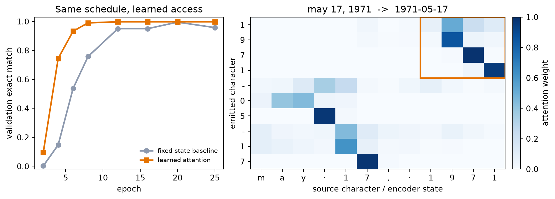

Figure 15.5: Left: exact-sequence accuracy on Chapter 13’s fixed 400-source validation subset. Both models use the same data, embedding and recurrent hidden widths, optimizer, top-level seed, and epoch schedule; attention adds parameters and a stepwise decoder, so this is not a parameter- or compute-matched ablation. Right: the predeclared first validation example. Rows are emitted ISO characters, columns are contextual encoder states indexed by source character, and the orange box marks the source year. The first four rows concentrate there.

At epoch 6, the fixed-state baseline is at \(53.75\%\) and the attentive model is at \(93.25\%\), a 39.5-point lead. At epoch 12 the comparison is \(95.0\%\) versus \(99.75\%\). The one final test audit is \(93.1\%\) versus \(100.0\%\) on 437 unambiguous sources.

WarningFaster convergence is not a one-variable proof

We matched examples, embedding and recurrent hidden widths, optimizer, top-level seed, number of updates, and epochs. We did not match parameter count, computation, or minibatch order: constructing models with different parameter counts consumes different random draws before their first permutation. The attentive model has 269,550 parameters versus 169,326, an increase of 59.2%, and its input-feeding decoder uses a Python step loop where Chapter 13’s teacher-forced baseline uses one fused target-sequence call. This one seeded synthetic run shows that the attention-equipped model reaches higher accuracy in fewer epochs and optimizer updates, not in less wall-clock time. It does not isolate bottleneck removal as the only possible cause.

The heatmap answers a narrower question. On the fixed validation example, the year must travel from the last four source positions to the first four outputs. The boxed region catches that movement, and across all 400 fixed validation examples, 97.5% of those four rows’ mass lands on states indexed by the source-year region. The top-weighted state is indexed inside that region 99.7% of the time.

NoteReading the heatmap

Columns are indexed by source characters, but their values are encoder states. Each state summarizes a recurrent prefix, so a delimiter can legitimately carry information about a field that just ended. Attention weights are internal allocation weights, not calibrated confidence and not a causal explanation of the model.

15.6 One head in the date model

The date model uses one learned additive scorer and one weighted context vector. Its query and key maps determine the scores; the encoder states themselves supply the values. In multi-head scaled dot-product attention, each head instead has its own query, key, and value projections. The head outputs are concatenated and passed through an output projection. Multi-head attention works for cross-attention as well as self-attention, and different heads can learn different relationships without any guarantee that they will. We keep one head here so its alignment stays easy to inspect. Chapter 16 derives the multi-head shapes and implements the full operator in its self-attention setting.

15.7 The bottleneck that remains

Cross-attention has repaired the fixed handoff. A decoder output can read any encoder state through one learned allocation. Yet both surrounding LSTMs remain recurrent: \(\vect{h}_i\) waits for \(\vect{h}_{i-1}\), and \(\vect{s}_t\) waits for \(\vect{s}_{t-1}\). Within either sequence, training cannot create all recurrent states at once.

The Q/K/V operator itself does not care where its three inputs came from. What if every position in one sequence supplied queries, keys, and values to every other position? Using self-attention in place of recurrence removes the sequential state update within each layer. It also changes how order enters the computation. Chapter 16 develops positional representations and distinguishes them from masks that restrict which positions may contribute.

NoteCheck yourself

Close the book for one minute and reconstruct the soft lookup.

• What distinct jobs do queries, keys, and values perform?
• Why does masking belong inside score normalization?
• What did making the compatibility function learnable buy over the fixed kernel?

15.8 Okay, so: attention softens the address

1. Attention softens the address. Chapter 13 learned embedding content while keeping lookup indices hard. Chapter 2’s softmax makes the lookup differentiable: learned scores become a distribution over memory locations.
2. Additive attention learns the compatibility function. Query and key enter a shared alignment space, tanh creates match features, and one selector produces each score. The same scorer is reused across all decoder/source pairs.
3. Scaled dot product learns comparison spaces. Projected \(\matr{Q}\matr{K}^{\top}/\sqrt{d_k}\) maps directly to dense matrix products. Under the idealized independent unit-variance model, scaling holds score variance near one instead of letting it grow with \(d_k\).
4. Masking is part of the operator. Padding is excluded before softmax; zero is not a mask. Cross-attention sees all real source positions, while causal masking belongs to the self-attentive decoder in Chapter 16.
5. On dates, attention learns where to read. Under the shared schedule, attention reaches 93.25% validation exact match at epoch 6 and 100.0% on the final test audit. Its year rows route 97.5% of validation weight to states indexed by the source-year region. Parameter count and compute were not matched: the attentive model has 59.2% more parameters.

The recurrent networks that write the memory stay in place for now; Chapter 16 lets a sequence query itself, so every position learns where to look and recurrence becomes optional.

Sources and further reading

• Bahdanau, Cho, & Bengio, Neural Machine Translation by Jointly Learning to Align and Translate: conjectures that the fixed-length encoder vector is a bottleneck, then tests differentiable soft search with an additive scorer.
• Luong, Pham, & Manning, Effective Approaches to Attention-based Neural Machine Translation: compares dot, general, and concat scoring functions and clarifies a second recurrent-attention timing convention.
• Vaswani et al., Attention Is All You Need: introduces scaled dot-product and multi-head attention in the architecture Chapter 16 builds.

Exercises

1. (Pencil.) Starting from Equation 15.2, write every batched shape for \(B=32\), source length 17, \(d_e=128\), \(d_d=96\), and \(d_a=64\). Which axis must softmax normalize, and why can the raw encoder and decoder widths differ?

2. (Code.) Extend the scaled-dot function with a deliberately all-false mask row. Confirm the guard catches it. Remove the guard and inspect the result of softmax over all \(-\infty\). Then replace the mask with zero scores and explain why padding receives weight.

3. (Pencil.) (a) Generalize the scaling derivation to independent coordinates with variances \(\sigma_q^2\) and \(\sigma_k^2\). (Code.) (b) Modify the seeded audit and check which divisor returns score variance near one.

4. (Code.) Replace the date model’s additive scorer with learned projected scaled-dot attention. Keep the split, schedule, and validation subset fixed. Select any design choices on validation, report the reused test endpoint once, and compare both convergence and year-region alignment. Explain why a large weight is neither calibrated confidence nor a causal explanation.

5. (Pencil.) The heatmap labels columns by source characters even though each value is a recurrent prefix state. Give two reasons a delimiter state might carry useful month or day information. Then state one conclusion the heatmap supports and one conclusion it cannot support.

6. (Audit.) The date model’s nn.Embedding learned a vector for each of the characters 0–9. Predict their geometry before looking. Named wrong answer: a clean number line ordered by numeric value, which is tempting but not what the training pressure rewards. Extract the ten rows, project them to two dimensions, and compare against the same rows from an untrained model (the falsifying control). What structure did training actually build, and which of the model’s jobs (months, days, years) explains it?

---

1. Appendix C turns that intuition into a conditional performance model: dense products can earn high arithmetic intensity through reuse, but shapes, data movement, implementation, and hardware decide the actual regime (Appendix C).

2. In Chapter 16, a feedforward network will help provide that nonlinear feature transformation after recurrence disappears.