5  Backpropagation

Chapter tools Lecture 2.1 · Backpropagation·Lecture 2.2 · Coding in PyTorch and Linear Regression with Autograd·Download notebook·Open in Colab (opens in a new tab)

Recall the update rule that ended Chapter 1: new parameters come from old parameters by stepping against the gradient, \(\vect{w}^{(t+1)} = \vect{w}^{(t)} - \eta\,\nabla_{\vect{w}}\loss\). For linear regression we could write that gradient down by hand. But a modern network has millions, sometimes billions, of knobs, tangled through layer after layer of composed functions, so computing each partial derivative separately, one extra forward pass per knob, is hopeless. Chapter 3 named the underlying difficulty: with no targets for the hidden units, how much of the output error should each hidden weight answer for? That is the credit assignment problem.

Backpropagation provides the exact algorithmic solution. It computes all the partial derivatives in one backward sweep whose cost is a small constant multiple of the forward graph’s operations. It is simply the multivariable chain rule in calculus but organized for computational reuse. We will derive it as a recursion on sensitivities, implement it from scratch on a batch, and analyze its arithmetic and memory costs.

5.1 One neuron, one chain

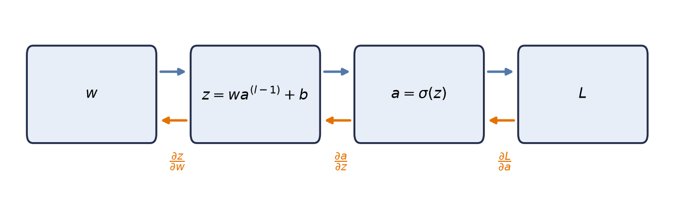
Start with the smallest possible case: one neuron on one training example. The previous activation \(a^{(l-1)}\) is multiplied by a weight \(w\), giving the pre-activation \(z = w\,a^{(l-1)} + b\); the activation function produces \(a^{(l)} = \sigma(z)\), written \(a\) below; and \(a\) feeds a loss \(L\).

Now turn the knob \(w\) a little. How much does \(L\) change? Follow the chain: turning \(w\) changes \(z\); the change in \(z\) changes \(a\); the change in \(a\) changes \(L\). The chain rule multiplies these local sensitivities:

\[ \frac{\partial L}{\partial w} = \frac{\partial L}{\partial a}\cdot \frac{\partial a}{\partial z}\cdot \frac{\partial z}{\partial w} . \tag{5.1}\]

Figure 5.1: Computation as a graph. The forward pass (top, blue) computes each value and keeps what the backward pass will reuse. The backward pass (bottom, dark red) starts from \(\partial L/\partial L = 1\) and multiplies one local derivative per edge, right to left. Each box on the lower lane is the loss’s sensitivity to the node above it; the one at \(z\) is the \(\delta\) of the next section.

Watch the mechanism: one knob, one chain

Turn w up by 0.01 — does the loss rise or fall, and by how much per unit of w?

These are this chapter's micro-autograd-check numbers, printed further down the chapter: w = 0.7, x = 2 in the place of the previous activation a^(l−1), b = −0.5, and the full squared error L = (a − y)² against y = 0.3. The four nodes on the line are the four boxes of the figure above.

\( \dfrac{\partial \residualpart{L}}{\partial \parameterpart{w}} \;=\; \class{oc-f3}{\residualpart{2(\predictionpart{a}-\targetpart{y})}}\cdot\class{oc-f2}{\predictionpart{\sigma'(z)}}\cdot\class{oc-f1}{\featurepart{x}} \;=\; \class{oc-f3}{\residualpart{0.821899}}\cdot\class{oc-f2}{\predictionpart{0.205500}}\cdot\class{oc-f1}{\featurepart{2}} \;=\; \class{oc-prod}{\residualpart{0.337801}} \)\[ \begin{aligned} \dfrac{\partial \residualpart{L}}{\partial \parameterpart{w}} &= \class{oc-f3}{\residualpart{2(\predictionpart{a}-\targetpart{y})}}\cdot\class{oc-f2}{\predictionpart{\sigma'(z)}}\cdot\class{oc-f1}{\featurepart{x}} \\ &= \class{oc-f3}{\residualpart{0.821899}}\cdot\class{oc-f2}{\predictionpart{0.205500}}\cdot\class{oc-f1}{\featurepart{2}} \\ &= \class{oc-prod}{\residualpart{0.337801}} \end{aligned} \]

Nothing was updated. Forward computes and keeps; backward reuses and multiplies.

The calculation is readable without playback. Opening this panel loads the optional controls.

One neuron, one example, one knob. Nothing is updated: no step is taken, no learning rate appears, and w ends where it started.

Scope and caveats

∂L/∂b, fan-out accumulation (a value used twice) and torch.autograd all come later in the chapter. The colours match the figure above: orange marks the one learnable knob this scene turns, and the backward pass is drawn in dark red, the colour these panels reserve for the loss and its sensitivities.

Check yourself. Same forward pass, same cache. What is the slope of the loss with respect to the bias b?

0.168900. The first two backward factors are reused unchanged, 0.821899 × 0.205500; only the last edge differs, because z changes by 1 per unit of b instead of x = 2 per unit of w. It is exactly half of the slope for w.

Transcript and keyboard help

1. One line, four nodes: w is a dial; z, a and L follow. Three fixed numbers sit on the edges: x = 2, b = −0.5, y = 0.3. Only w turns. Before playing: turn w up by 0.01 — does L rise or fall, and by how much per unit of w?
2. Forward, left to right. w = 0.700 gives z = 0.900, then a = σ(z) = 0.710950, then L = (a − y)² = 0.168879. Each value is computed from the one before it and kept.
3. The dial turns to 0.710 and a nudge of +0.010 leaves it. Through z = wx + b it doubles: Δz = +0.020 (z reads 0.920). Through σ it shrinks about five-fold: Δa = +0.004093 (a reads 0.715042). Through (a − y)² it shrinks a little more: ΔL = +0.003380 (L reads 0.172260).
4. Measured: 0.003380 per 0.010, so ΔL/Δw = 0.338046 per unit of w. That is the number the backward pass has to reproduce.
5. The dial returns to 0.700 and every value returns with it; the ghosts of the nudge stay. The backward pass leaves L and walks back the last edge: its slope is 2(a − y) = 2 × 0.410950 = 0.821899, read off the kept a.
6. Back one more edge: the slope of σ at the kept z is a(1 − a) = 0.710950 × 0.289050 = 0.205500 — from the kept value, not the turned one.
7. Back to w: the slope of wx + b in w is x = 2.
8. Multiply the three: 0.821899 × 0.205500 × 2 = 0.337801, written under the measured 0.338046. They agree to three decimals. A finite difference is not the derivative; it is the derivative plus a term that shrinks with Δw.
9. Nothing was updated: w is where it started. Forward computes and keeps; backward reuses and multiplies.

Silent; paused initially; 1.5× playback. Focus the animation pane: Space or K plays/pauses, arrows seek between the nine beats, Home/End jump, Escape pauses. The scrubber and speed menu also work by keyboard. Reduced-motion mode holds each beat’s state: the dial snaps to 0.710, the nudge stands at L with all four ghosts already drawn, and each backward ray arrives whole at its own beat instead of travelling.

Two things about this picture generalize to any network, however deep:

1. The forward pass caches. Computing \(L\) produces the intermediate values (\(z\), \(a\)) along the way; we keep them, because the backward pass will need them.
2. The backward pass reuses. It uses cached values, multiplying local derivatives along each path and summing contributions from multiple paths. The whole sweep costs a small constant multiple of one forward pass; for matrix-multiply layers the multiple is about two, as the batched code below makes visible.

5.2 Sensitivity propagation: the four layer equations

For a full layer of neurons the bookkeeping threatens to become a tangled mess of sums. The cure is to choose one intermediate quantity per layer and track only that. At the output, the loss is an explicit function of the network’s last values; for a weight ten layers deep, the dependence runs through every layer in between. Backpropagation carries the loss’s sensitivity from the output, where it is explicit, back to each layer that needs it.

NoteThe layer sensitivity

Define, for each layer \(l\), the sensitivity

\[ \delta^{(l)} \;:=\; \frac{\partial L}{\partial \vect{z}^{(l)}} , \]

the gradient of the loss with respect to that layer’s pre-activations. Entry \(j\) has a first-order meaning: if \(z^{(l)}_j\) moved by a small \(\varepsilon\), the loss would move by about \(\delta^{(l)}_j\,\varepsilon\). Automatic differentiation calls such a quantity an adjoint: the derivative of the final output with respect to an intermediate value, computed backward from the output.

For fully connected layers with elementwise activation functions, backpropagation takes the following four forms. Here \(\odot\) denotes the elementwise (Hadamard) product.

1. Start at the output layer \(L\), where the sensitivity is explicit:

\[ \delta^{(L)} = \frac{\partial L}{\partial \vect{a}^{(L)}} \odot \sigma'(\vect{z}^{(L)}) . \tag{5.2}\]

For the half-squared-error convention \(L=\tfrac12\|\vect{a}^{(L)}-\vect{y}\|^2\), \(\partial L / \partial \vect{a}^{(L)}\) is exactly the prediction error \(\vect{a}^{(L)} - \vect{y}\). Other conventions contribute a known scale: mean squared error, for example, contributes \(2/n\) for \(n\) scalar outputs. In every case the output error is then multiplied by the activation derivative, which measures how sensitive the activation was to its input.

2. Propagate one layer back:

\[ \delta^{(l)} = \Bigl( (\matr{W}^{(l+1)})^\top \delta^{(l+1)} \Bigr) \odot \sigma'(\vect{z}^{(l)}) . \tag{5.3}\]

The sensitivity travels backward through the same weights the signal traveled forward through. Unit \(j\) of layer \(l\) fed every unit \(i\) of layer \(l+1\) through the weight \(W^{(l+1)}_{ij}\), so it collects \(\sum_i W^{(l+1)}_{ij}\,\delta^{(l+1)}_i\), which is entry \(j\) of \((\matr{W}^{(l+1)})^\top\delta^{(l+1)}\): hence the transpose. The activation derivative \(\sigma'(\vect{z}^{(l)})\) then scales it. This recursion runs from the last layer to the first.

1. Fix the seed, draw weights for layer sizes 3, 4, 4, 1 and one input, and start an empty cache.
2. Cache the forward pass, then apply equations 1 and 2 from the output back.

import torch
import matplotlib.pyplot as plt
torch.set_num_threads(4)  # pinned: results depend on the CPU thread count

# [1]
torch.manual_seed(6050)
sizes = [3, 4, 4, 1]
Ws = [torch.randn(sizes[i + 1], sizes[i]) for i in range(3)]

x = torch.randn(3)                       # forward pass, cached
zs, a = [], x
# [2]
for W in Ws[:-1]:                        # hidden layers: sigmoid
    zs.append(W @ a)
    a = torch.sigmoid(zs[-1])
zs.append(Ws[-1] @ a)                    # identity output, as in our 2-layer build

delta = [None] * 3                       # backward pass: eqs. 1 and 2
sp = lambda z: torch.sigmoid(z) * (1 - torch.sigmoid(z))
delta[2] = zs[2] - 1.0                               # eq. 1 (identity output, y = 1)
delta[1] = (Ws[2].T @ delta[2]) * sp(zs[1])          # eq. 2
delta[0] = (Ws[1].T @ delta[1]) * sp(zs[0])          # eq. 2 again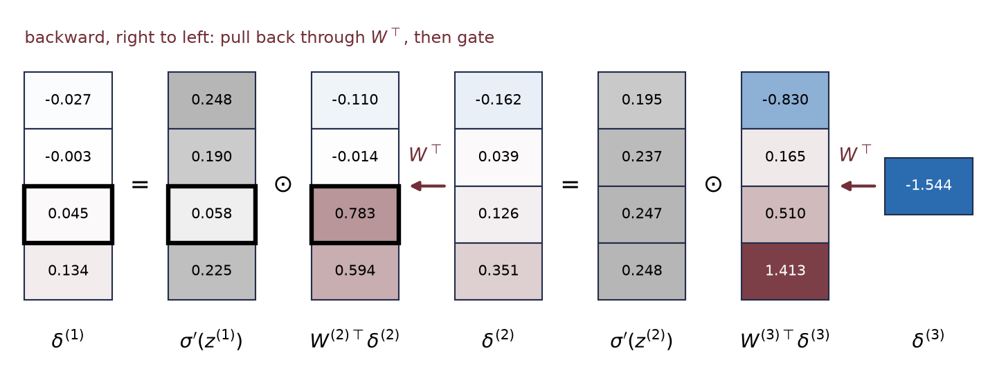

Figure 5.2: Equation 5.3 as two operations, run right to left on a 3–4–4–1 network (random weights, one example): multiply by \(W^\top\), which sends each sensitivity back to every unit that fed it, then multiply elementwise by the activation derivative \(\sigma'(z) \le 0.25\) (gray). The numbers are the executed values; blue is negative and dark red positive on one shared scale, so the fading toward the input shows the derivatives at work. The outlined row has the smallest derivative: a large pulled-back value leaves it as a small sensitivity.

3. Convert sensitivities into weight gradients:

\[ \frac{\partial L}{\partial \matr{W}^{(l)}} = \delta^{(l)} \, (\vect{a}^{(l-1)})^\top . \tag{5.4}\]

4. And into bias gradients:

\[ \frac{\partial L}{\partial \vect{b}^{(l)}} = \delta^{(l)} . \tag{5.5}\]

Check the shapes in Equation 5.4. With \(m\) neurons in layer \(l\) and \(k\) in layer \(l-1\), \(\delta^{(l)}\) is \((m \times 1)\), and \((\vect{a}^{(l-1)})^\top\) is \((1 \times k)\). Their outer product is an \(m \times k\) matrix, exactly the shape of \(\matr{W}^{(l)}\), and entry \((i,j)\) is the sensitivity of neuron \(i\) times the activation of neuron \(j\) that fed it, \(\partial L/\partial W^{(l)}_{ij} = \delta^{(l)}_i\,a^{(l-1)}_j\). A weight’s gradient is sensitivity out times signal in:

1. Form the weight-gradient outer product.

# [1]
d2 = delta[1]                              # layer-2 sensitivity  (4,)
a1 = torch.sigmoid(zs[0])                  # layer-1 activations  (4,)
G = torch.outer(d2, a1)                    # eq. 3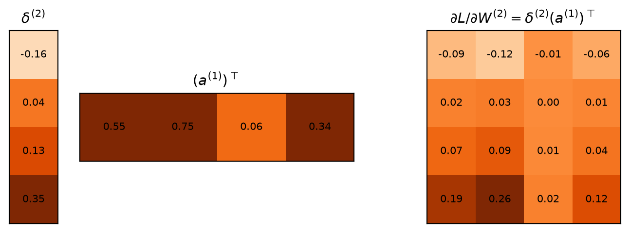

Figure 5.3: Equation 5.4 with the sensitivities and activations from the network above: a \((4 \times 1)\) sensitivity column times a \((1 \times 4)\) activation row gives the whole \((4 \times 4)\) gradient at once. The outlined cells trace the largest entry, \(\delta_i\,a_j\); every other cell is built the same way. Sensitivities and gradients share the signed blue-to-dark-red scale; the activations, all positive, are green.

The matrix form needs no explicit summations, and it maps directly onto the parallel matrix multiplies that GPUs are built for. The same reverse-mode principle applies to larger models, using the local derivative of each operation.

5.3 Manual implementation and autograd verification

We implement the four equations on a two-layer network using basic tensor operations, with no autograd involved, and then run PyTorch’s autograd on the same network. If the derivation and tensor shapes are correct, the two sets of gradients agree to machine precision.

1. Load the chapter dependencies and establish reproducible state.

import torch

# [1]
_ = torch.manual_seed(6050)

The code makes one change of layout: it processes \(n\) examples at once, stored as rows as in Chapter 1. Stack the activations into \(\matr{A}^{(l-1)} \in \mathbb{R}^{n\times k}\) and the sensitivities into \(\matr{\Delta}^{(l)} \in \mathbb{R}^{n\times m}\), row \(i\) holding example \(i\)’s \(\delta^{(l)}\). The single-example outer product of Equation 5.4 then becomes one matrix product that sums the per-example outer products,

\[ \frac{\partial L}{\partial \matr{W}^{(l)}} = (\matr{\Delta}^{(l)})^\top \matr{A}^{(l-1)} = \sum_{i=1}^{n} \delta^{(l)}_i \,(\vect{a}^{(l-1)}_i)^\top , \]

and Equation 5.3, transposed row by row, becomes \(\matr{\Delta}^{(l)} = \bigl(\matr{\Delta}^{(l+1)}\matr{W}^{(l+1)}\bigr) \odot \sigma'(\matr{Z}^{(l)})\), with the pre-activations stacked into \(\matr{Z}^{(l)}\) in the same way. The mean’s \(1/n\) already sits inside \(\matr{\Delta}^{(2)}\), so the sum is the batch average.

1. Draw a batch of 32 inputs and targets and the two-layer weights.
2. Cache the forward pass, propagate the sensitivities backward, and form the gradients.
3. Rebuild the network from requires_grad copies and let autograd differentiate it.
4. Print the largest gap between each hand-computed gradient and autograd’s.

# [1]
n, d, h = 32, 5, 8                            # batch, input dim, hidden dim
X = torch.randn(n, d)
y = torch.randn(n)

W1, b1 = torch.randn(h, d) * 0.3, torch.zeros(h)
W2, b2 = torch.randn(1, h) * 0.3, torch.zeros(1)

# [2]
# forward pass -- cache everything the backward pass will need
Z1 = X @ W1.T + b1                            # (n, h)
A1 = torch.sigmoid(Z1)                        # (n, h)
Z2 = A1 @ W2.T + b2                           # (n, 1)
L = ((Z2.squeeze() - y) ** 2).mean()

# backward pass -- the four equations (batch-averaged)
sig_prime = A1 * (1 - A1)                     # sigma'(z) = sigma(z)(1 - sigma(z))
delta2 = 2 * (Z2.squeeze() - y)[:, None] / n  # eq. 1 (identity output: no gate)
delta1 = (delta2 @ W2) * sig_prime            # eq. 2: back through W^T, then gated
grads = {                                     # eqs. 3 & 4: sensitivity out x signal in
    "W2": delta2.T @ A1, "b2": delta2.sum(0),
    "W1": delta1.T @ X,  "b1": delta1.sum(0),
}

# [3]
# same network, autograd's turn
params = {k: v.clone().requires_grad_(True) for k, v in
          {"W1": W1, "b1": b1, "W2": W2, "b2": b2}.items()}
A1_ = torch.sigmoid(X @ params["W1"].T + params["b1"])
L_ = (((A1_ @ params["W2"].T + params["b2"]).squeeze() - y) ** 2).mean()
L_.backward()

# [4]
for k in grads:
    gap = (grads[k] - params[k].grad).abs().max()
    print(f"{k}: max |ours - autograd| = {gap:.2e}")

W2: max |ours - autograd| = 0.00e+00
b2: max |ours - autograd| = 0.00e+00
W1: max |ours - autograd| = 3.73e-09
b1: max |ours - autograd| = 1.86e-09

The largest discrepancy is \(3.73\times10^{-9}\), consistent with float32 rounding. The four equations are what autograd computes; the framework simply builds the computation graph for us as we go and then walks it backward, caching and reusing as we did.

Two products backward for each product forward. The forward pass computed the output layer with one matrix product, \(\matr{A}^{(1)}(\matr{W}^{(2)})^\top\). Its backward pass needed two, one for each input of that product: \(\matr{\Delta}^{(2)}\matr{W}^{(2)}\) carries the sensitivity to the layer’s input, and \((\matr{\Delta}^{(2)})^\top\matr{A}^{(1)}\) forms the weight gradient. For an \(n\times k\) input and an \(m\times k\) weight, each of the three products costs \(2nmk\) floating-point operations, so a matrix-multiply layer’s backward pass costs about twice its forward pass and a training step about three forward passes. That is the small constant multiple stated at the start of the chapter. (The first layer needs no input gradient, because nothing upstream of the input \(\matr{X}\) is trained; our code never forms one.)

Caching costs memory. The backward pass read the hidden activations \(\matr{A}^{(1)}\), for the activation derivative \(\sigma'(\matr{Z}^{(1)})\) and the gradient of \(\matr{W}^{(2)}\), and the input \(\matr{X}\), for the gradient of \(\matr{W}^{(1)}\), so both had to survive the forward pass. Here \(\matr{A}^{(1)}\) alone holds \(32 \times 8 = 256\) numbers, more than all \(57\) parameters of the network, and it grows with the batch size while the parameter count does not. A deep network keeps about one such block per layer until the backward pass consumes it, which is why training a network takes more memory than running it, and why evaluation code runs under torch.no_grad(), where no graph is recorded and nothing is kept for a backward pass. Recomputing some activations during the backward pass instead of storing them, gradient checkpointing, trades extra arithmetic for memory (Chen et al., 2016).

5.4 Order and accumulation: how autograd traverses graphs

The four layerwise equations derived above assume a strictly sequential network, where each layer feeds exactly one successor. Real computational workflows form directed acyclic graphs (DAGs): a single intermediate value may branch into multiple downstream operations. Extending reverse-mode differentiation to arbitrary DAGs requires two rules:

1. Reverse topological ordering. The backward sweep must visit nodes in reverse topological order, ensuring every downstream consumer of an intermediate tensor has finished propagating its sensitivity before that tensor sends its own gradient upstream.
2. Gradient accumulation. When an intermediate variable branches into multiple operations, the multivariable chain rule dictates that its total sensitivity is the sum of the sensitivities along each path. Autograd engines therefore accumulate adjoint contributions using addition rather than overwriting.

A small engine shows both rules. Each Value node records its parents and a local derivative rule; its grad field holds its adjoint \(\partial L/\partial v\), and the rule passes that adjoint on to the parents.

This teaching implementation is adapted from Andrej Karpathy’s micrograd, released under the MIT License. We use only the scalar reverse-mode pattern, as a readable model of these two rules; the upstream copyright and license notice are preserved in the repository’s third-party notices.

1. Implement scalar reverse-mode autodiff with a topological backward traversal.

# [1]
class Value:
    """A scalar that remembers its history -- a node in the computation graph."""

    def __init__(self, data: float, parents=(), backward_rule=lambda: None):
        self.data = data
        self.grad = 0.0
        self._parents = parents
        self._backward_rule = backward_rule

    def __add__(self, other: "Value | float") -> "Value":
        other = other if isinstance(other, Value) else Value(other)
        out = Value(self.data + other.data, (self, other))
        def rule():                      # d(out)/d(self) = d(out)/d(other) = 1
            self.grad += out.grad
            other.grad += out.grad
        out._backward_rule = rule
        return out

    def __mul__(self, other: "Value | float") -> "Value":
        other = other if isinstance(other, Value) else Value(other)
        out = Value(self.data * other.data, (self, other))
        def rule():                      # product rule, one side at a time
            self.grad += other.data * out.grad
            other.grad += self.data * out.grad
        out._backward_rule = rule
        return out

    def sigmoid(self) -> "Value":
        s = 1 / (1 + 2.718281828459045 ** (-self.data))
        out = Value(s, (self,))
        def rule():                      # sigma' = s (1 - s), the gate
            self.grad += s * (1 - s) * out.grad
        out._backward_rule = rule
        return out

    def backward(self) -> None:
        order, seen = [], set()
        def topo(v):                     # creators land in order first
            if v not in seen:
                seen.add(v)
                for p in v._parents:
                    topo(p)
                order.append(v)
        topo(self)
        self.grad = 1.0                  # dL/dL = 1: seed the output adjoint
        for v in reversed(order):
            v._backward_rule()

1. Build one sigmoid neuron from Value nodes and its squared error against the target 0.3.
2. Call loss.backward() to fill every node’s grad.
3. Print the engine’s dL/dw beside the same derivative from the hand formula.

# [1]
w, x, b = Value(0.7), Value(2.0), Value(-0.5)
a = ((w * x) + b).sigmoid()             # one neuron, forward
loss = (a + (-0.3)) * (a + (-0.3))      # squared error vs target 0.3
# [2]
loss.backward()

# analytic check: dL/dw = 2(a - y) * sigma'(z) * x
z = 0.7 * 2.0 - 0.5
s = 1 / (1 + 2.718281828459045 ** (-z))
# [3]
print(f"micro-autograd: dL/dw = {w.grad:.6f}")
print(f"by hand:        dL/dw = {2 * (s - 0.3) * s * (1 - s) * 2.0:.6f}")

micro-autograd: dL/dw = 0.337801
by hand:        dL/dw = 0.337801

The check exercised both rules. The loss writes a twice, in both factors of (a + (-0.3)) * (a + (-0.3)), so a.grad is the sum of two contributions, and the sort guarantees that both arrive before a’s own rule passes the total on toward w. PyTorch’s autograd keeps the same two rules and changes the unit of work: its nodes hold tensors, and each local rule is a vector–Jacobian product, which maps the adjoint of an output to the adjoints of the inputs without ever forming a Jacobian. For the layer product \(\matr{Z} = \matr{A}\matr{W}^\top\), the rule is the pair from the batched code, \(\bar{\matr{A}} = \bar{\matr{Z}}\matr{W}\) and \(\bar{\matr{W}} = \bar{\matr{Z}}^\top\matr{A}\), where a bar marks an adjoint. The scalar engine models the bookkeeping, not the speed.

Watch the mechanism: one value, two branches, one counter

The chapter's squared error writes a twice, so its gradient comes back along two edges. Does the counter on a end up holding one arrival or the sum of both?

The backward pass of the chapter's own autograd check, drawn from the branch down: one activation feeding two copies of the same subtraction, and the running total the engine keeps with +=.

\( \loss = \class{bb-product}{u\,v}, \qquad u = v = \predictionpart{a} - \targetpart{0.3} \)\( \residualpart{\dfrac{\partial \loss}{\partial \predictionpart{a}}} = \class{bb-first}{\dfrac{\partial \loss}{\partial u}\dfrac{\partial u}{\partial \predictionpart{a}}} \class{bb-plus}{+} \class{bb-second}{\dfrac{\partial \loss}{\partial v}\dfrac{\partial v}{\partial \predictionpart{a}}} \)

Two uses, two arrivals, one sum. That is where the factor of two comes from.

The calculation is readable without playback. Opening this panel loads the optional controls.

This is the backward pass of one already-written expression: nothing here is trained, no weight is updated, and the forward values are the chapter's own.

Scope and caveats

The picture starts below the neuron. The chapter's forward pass runs w, x and b through a sigmoid to reach a; that single chain is the one-chain excerpt, which names branch accumulation as the thing it leaves out. This panel picks the derivative up at a and puts the trunk back in only at the end, as one grey factor, so that the arithmetic lands on the gradient the chapter prints.

The two subtraction nodes are drawn apart because the chapter's line evaluates (a + (-0.3)) twice and the engine therefore builds two nodes, each recording a as a parent. Written once and multiplied by itself, it would be a single node with the same parent recorded twice, and the accumulation would be identical: the product rule adds one contribution per recorded use, not one per line of source.

The hollow bar under the meter is a counterfactual, not a second model: it marks where the counter would stop if the rules assigned with = instead of accumulating with +=, and the struck number beside it is what the chapter would then have printed. Every value shown is recomputed from the declared inputs with the chapter's own value of e, at four decimal places; the loss value itself is never drawn, because only its seed of one enters the backward pass. Green is the activation the chapter computes, purple the target it is compared against, wine the gradient travelling back, orange the learnable weight, grey the scenery and the trunk.

Check yourself. Change one digit so the second subtraction takes 0.1 away instead of 0.3 — the same activation, two different targets. What does the counter on a read now, and is it still twice one branch?

1.0219, and no. The product rule sends each branch the other branch's value, so the upper edge carries 0.6109 and the lower carries 0.4109, and the counter holds their sum. Doubling was never the rule; it was what equal branches happened to give. The trunk then prints 0.4200 instead of 0.3378.

Transcript and keyboard help

1. Predict. The activation a holds 0.7109. Two nodes below it each compute a minus the target 0.3, and both give 0.4109; one product node multiplies them. The counter on a is empty. The gradient is about to come back along two edges: will the counter hold one arrival or both?
2. Seed the loss. The backward pass sets the loss's own gradient to 1, the line the chapter comments as seeding the output adjoint. The product rule is about to send each branch the other branch's value.
3. The first branch arrives. A packet of 0.4109 leaves the product along the upper edge, passes through the upper subtraction unchanged, and is added into the counter on a, which reads 0.4109.
4. Hold. The second packet is still waiting at the product node, carrying the same 0.4109. The counter still reads one arrival. Predict what it will read once the second lands.
5. The second branch arrives. The packet travels the lower edge and is added into the same counter, which now reads 0.8219 — the sum, not the last value. This is the plus in the engine's plus-equals.
6. What assignment would have cost. A hollow bar grows back out to 0.4109: the reading the counter would have kept if the rules had written a plain equals. The meter itself does not move; the real total stands.
7. Down the trunk. The accumulated 0.8219 is multiplied by the sigmoid's own slope 0.2055 and by the input 2, and lands on 0.3378 — the gradient the chapter prints as 0.337801.
8. Compare. Beside it, struck through, is 0.1689: what the same trunk would have produced from a single arrival. Two uses, two arrivals, one sum, and the factor of two in the derivative of a square.

Silent; paused initially; 1.5× playback. Focus the animation pane: Space or K plays/pauses, arrows seek between beats, Home/End jump, Escape pauses. The scrubber and speed menu also work by keyboard. Reduced-motion mode holds each beat's finished state instead of moving between them.

5.5 PyTorch autograd in practice: five rules

Autograd uses the same reverse pass we built manually. Understanding that pass explains its practical rules. These five cover nearly every autograd bug you will meet; Figure 5.4 pictures four of them in PyTorch syntax.

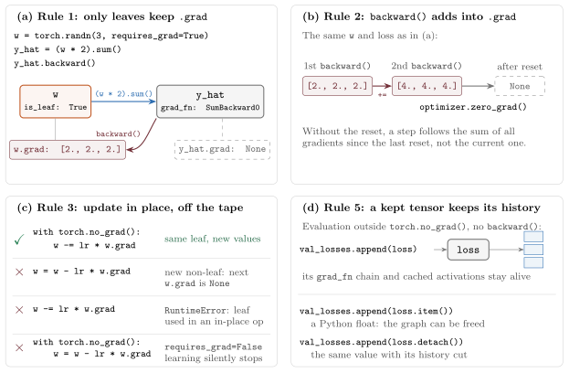
Figure 5.4: Four autograd rules in PyTorch syntax. (a) After the backward pass, the leaf w holds its gradient; the non-leaf y_hat used its gradient and released it. (b) A second backward pass adds into w.grad until optimizer.zero_grad() resets it. (c) Of four ways to write an update, only the in-place one with recording paused keeps w a trainable leaf. (d) A loss stored from a forward pass that is never backpropagated keeps its graph and cached activations alive; loss.item() and loss.detach() keep only the value.

Rule 1: by default, only leaf tensors retain gradients. A leaf is a tensor you created directly (your parameters); a non-leaf is the result of an operation (activations, losses). After the backward pass, each leaf holds its gradient in the attribute .grad, while intermediate gradients are used and released. Call .retain_grad() on a non-leaf before the backward pass only when you explicitly need its gradient for inspection.

Rule 2: gradients accumulate. Each backward pass adds into the gradient attribute. Zero the gradients before each step (optimizer.zero_grad()), or every update uses the sum of all past gradients.

1. Create a leaf parameter w and a non-leaf output y_hat computed from it.
2. Backpropagate twice without clearing the leaf gradient.
3. Print the leaf and non-leaf gradients, then call backward() on a rebuilt sum and reprint w.grad.

# [1]
w = torch.randn(3, requires_grad=True)      # leaf: our parameter
y_hat = (w * 2).sum()                       # non-leaf: result of an operation

# [2]
y_hat.backward()
# [3]
print(f"leaf grad:      {w.grad.tolist()}")            # populated
print(f"non-leaf grad:  {y_hat.grad}")                 # None -- rule 1

(w * 2).sum().backward()                    # backward again, WITHOUT zeroing
print(f"after 2nd pass: {w.grad.tolist()}")            # doubled -- rule 2

leaf grad:      [2.0, 2.0, 2.0]
non-leaf grad:  None
after 2nd pass: [4.0, 4.0, 4.0]

Rule 3: update parameters in place, with recording paused. Write the update as w -= lr * w.grad inside with torch.no_grad():. Both halves matter. Pausing the recording keeps the step itself off the graph, and the in-place subtraction changes the values of the existing leaf, so w remains the same trainable tensor that the optimizer and the next backward pass refer to. Drop either half and the update breaks (Figure 5.4, panel c): the rebinding w = w - lr * w.grad creates a new non-leaf whose gradient is not populated on the next pass; an in-place update with recording on raises an error; and a rebinding with recording paused yields a tensor that no longer requires gradients, so learning silently stops. Assigning a plain tensor to a registered module parameter fails loudly instead. The idiom:

1. Save the leaf parameter and choose a learning rate.
2. Pause graph recording and update the parameter in place.
3. Verify that the update changed the value without changing leaf status.

# [1]
before = w.detach().clone()
lr = 0.1

# [2]
with torch.no_grad():
    w -= lr * w.grad

# [3]
assert not torch.equal(w, before)
assert w.is_leaf

Rule 4: in-place operations can corrupt the backward pass. Methods ending in _ (add_, relu_) overwrite values that the backward pass may still need from the forward cache. They are safe in parameter updates with recording paused; anywhere else, prefer creating a new tensor.

Rule 5: stored tensors can retain computation graphs. Every forward pass builds a fresh graph, and the backward pass frees the activations that graph cached. A tensor you keep, say the loss appended to a list for plotting, still holds a reference to the graph that produced it; one kept from a forward pass that is never backpropagated (an evaluation loop that leaves recording on, for example) holds every cached activation as well. Store loss.item() (a plain float) or loss.detach() instead: the detached tensor has the same value and no reference to the graph.

WarningKeep updates outside the graph

The one safe manual update is in place and unrecorded: w -= lr * w.grad inside with torch.no_grad():, then clear the leaf’s gradient (Rule 2) before the next backward pass. Rules 1 and 3 combine into the classic raw-tensor bug: the rebinding w = w - lr * w.grad creates a new non-leaf, and its .grad comes back None on the next pass.

5.6 Activation derivatives and depth

In Equation 5.3, the transposed weight matrix combines sensitivities from the next layer, and the activation derivative scales each resulting component. A derivative near zero attenuates that component; a derivative equal to one leaves it unchanged at this operation.

For the logistic sigmoid, \(\sigma'(z) = \sigma(z)(1-\sigma(z))\). Its maximum value, at \(z = 0\), is exactly \(0.25\); as the activation saturates toward either endpoint, its derivative approaches zero.

1. Evaluate the sigmoid and ReLU derivative gates.

import matplotlib.pyplot as plt

# [1]
z = torch.linspace(-6, 6, 300)
sig = torch.sigmoid(z)
sigmoid_gate = sig * (1 - sig)
relu_gate = (z > 0).float()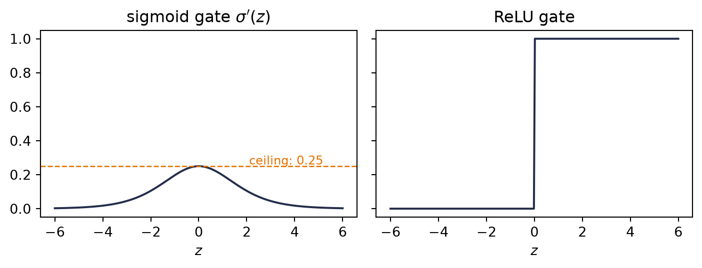

Figure 5.5: Activation derivatives on a common vertical scale. The sigmoid derivative never exceeds \(0.25\) and approaches zero under saturation. The ReLU derivative is zero for negative inputs and one for positive inputs.

Watch the mechanism: active forward, quiet backward

Can a neuron have a large output and still pass almost no backward sensitivity?

Watch one activation component in both directions. Its face is its own activation curve: the operating point rides that curve, and the tangent drawn there is the multiplier a backward unit probe meets. The timeline moves z; you can drag it too.

z

−6−3036

z = 6

\( \residualpart{g_z}=\residualpart{g_a}\,\class{dg-local-factor}{f'(z)} \) \( \sigma'(z)\leq\class{dg-quarter}{\tfrac14},\quad \operatorname{ReLU}'(z)=\class{dg-open}{1}\ (z>0) \) \( \prod_{j=1}^{k}\sigma'(z_j)\leq\class{dg-quarter}{(\tfrac14)^k} \)

Ten best-case sigmoid gates: below one millionth, yet not zero. Weights and branching, omitted here, also scale the full gradient.

The calculation is readable without playback. Opening this panel loads the optional controls.

The unit probe measures a local sensitivity, not an observed loss gradient.

Scope and caveats

Filled area is proportional to that sensitivity; the hollow ring only locates a signal that may be too small to see. The component's face shows its activation function on that function's own vertical scale (sigmoid from 0 to 1, ReLU from 0 to 6), so a tangent's tilt compares slopes within one face, not across the two; the printed multiplier is the number. The z slider covers the chapter's plotted domain, from −6 to 6: every value at a dragged z is computed from the chapter's formulas, not printed in it. The ten-component path isolates best-case sigmoid derivative factors, not ten simulated forward activations. Its ruler is a logarithmic scale, a drawing device: multiplying by one quarter is one equal step of log₁₀(¼), and the active-ReLU mark stays at 1 because each active factor is one. Weight matrices and branching are omitted from this ceiling, not assumed harmless: they also affect the complete backward recursion. Active ReLU contributes one locally; negative inputs contribute zero. At its nondifferentiable zero, PyTorch chooses zero for backpropagation, a convention and not a slope, so no tangent is drawn there. Nothing is trained or updated.

Check yourself. At z = −6 the sigmoid's output is about 0.0025: a quiet neuron. What is its backward factor?

About 0.0025 again: the sigmoid's slope at −6 equals its slope at +6, 0.002467. The slope is what matters, and the S is flat at both ends. Sensitivity peaks at z = 0, where the factor is exactly ¼.

Transcript and keyboard help

1. The picture is an activation component inside a network: the weighted sum supplies pre-activation z; the component emits a for the next layer. The component's face is its own activation curve between two dotted rails, the output's floor and ceiling, with no grid. At z=0 the operating point sits mid-curve and the sigmoid emits one half.
2. Keep that forward value cached. A tangent appears at the operating point, tied by a dashed link to the multiplier on the backward lane, which reads "times slope". A normalized unit sensitivity then travels from the output side toward the input side. This probe isolates the activation derivative; it does not cross an uncomputed weight matrix. The slope stays withheld until the probe meets the multiplier.
3. At the component the filled signal area becomes one quarter of its incoming area. The derivative at zero is exactly one quarter even though the manuscript's even-sized 300-point plotting grid does not sample zero. Then z rises toward six: the point rides up the curve, the output grows, the tangent tilts flat, and the multiplier returns to a question mark.
4. At z=6 the sigmoid output is approximately 0.9975 and the tangent is nearly flat. Predict the backward multiplier before watching the probe return.
5. The same unit probe is now multiplied by approximately 0.002467. The large forward output stays visible. A large activation does not imply a large local derivative: activity and sensitivity are different quantities. Dragging z to minus six shows the other side: output near zero and the same tiny slope, quiet forward and quiet backward.
6. Substitute ReLU at the same positive input. Its face is a line with an explicit vertex at zero; its output is six and its slope is one, so the unit backward probe passes unchanged. For a negative input the slope is zero and nothing is delivered. At the kink no tangent is drawn: PyTorch's zero there is a convention, not a classical derivative. This is not a guarantee about surrounding weights.
7. Return to the sigmoid witness and isolate only the sigmoid factors along a longer backward path. The numbered components count factors in reverse traversal order, not measured network layers. Each is given its largest possible multiplier, one quarter; the weight-matrix contributions are outside this calculation. Under the path a logarithmic ruler runs from 1 on the right past ten to the minus six on the left. Each crossing moves its marker one equal step left, because multiplying by a constant is an equal step on a log scale. A second mark, the active-ReLU path, stays at 1.
8. Ten such factors give at most 1/1,048,576, approximately 9.54 times ten to the minus seven: ten equal steps, ending just past the ten-to-the-minus-six tick. The filled signal is still positive even when it becomes subpixel; its outline is only a location cue. This ceiling is not a bound on the complete gradient. The manuscript's separate experiment measures actual networks.

Silent; paused initially; 1.5× playback. Focus the animation pane: Space or K plays/pauses, arrows seek between beats, Home/End jump, Escape pauses. The scrubber and speed menu also work by keyboard. The z slider is the one parameter control: the timeline moves it, and dragging it pauses playback and recomputes the whole picture from your z; its arrow keys change z by 0.1 and never seek the timeline. Play, a scrub or a beat key returns z to the timeline. Reduced-motion mode holds each beat's state instead of moving between them.

Products of these derivatives produce one of the central failure modes of deep networks. The chain rule multiplies local Jacobians across layers. The activation-derivative part of a sigmoid path contributes at most \(0.25\) per layer, so that part is bounded by \(0.25^k\) after \(k\) gates. Ten gates in, its ceiling is below one in a million. The weight matrices and branching paths also scale the full network Jacobian, so \(0.25^k\) bounds the activation-derivative product alone, not the complete gradient; it isolates why repeated sigmoid derivatives strongly favor vanishing signals.

Now replace the sigmoid with ReLU. \(\mathrm{ReLU}(z) = \max(0, z)\) has derivative \(1\) for \(z > 0\) and \(0\) for \(z < 0\). At the kink \(z=0\), PyTorch uses derivative \(0\); exact zeros can occur with zero biases or sparse activations. The derivative is either one or zero. At an active unit the sensitivity passes through this factor unchanged; the surrounding weight matrices can still amplify or attenuate it, which is where the weight scale comes in.

We test the argument in two networks that differ only in the activation function. Both have 30 layers, one with sigmoid units and one with ReLU. Both get the same He-scaled weights and input batch, and we record how much gradient reaches each layer. We compute the diagnostic in float64 so the norm itself does not underflow; then we ask the practical float32 question: would a learning-rate-\(0.1\) update actually change the first layer’s stored weights?

1. Define the reusable gradient_diagnostic helper.
2. Start an empty diagnostics dictionary and open the figure.
3. Implement the depth experiment.
4. Show the plot, then print each network’s first-layer max gradient and its nonzero and changed counts.

from torch import nn

# [1]
def gradient_diagnostic(
    activation: type[nn.Module], depth: int = 30, width: int = 64
) -> dict[str, object]:
    torch.manual_seed(6050)
    layers = []
    for _ in range(depth):
        layers += [nn.Linear(width, width), activation()]
    net = nn.Sequential(*layers, nn.Linear(width, 1)).double()
    with torch.no_grad():
        for layer in net:
            if isinstance(layer, nn.Linear):
                nn.init.normal_(layer.weight, std=(2 / layer.in_features) ** 0.5)
                nn.init.zeros_(layer.bias)

    out = net(torch.randn(128, width, dtype=torch.float64)).mean()
    out.backward()
    linears = [layer for layer in net if isinstance(layer, nn.Linear)][:-1]
    first = linears[0]
    grad32 = first.weight.grad.float()
    weight32 = first.weight.detach().float()
    changed = ((weight32 - 0.1 * grad32) != weight32).sum().item()
    return {
        "norms": [layer.weight.grad.norm().item() for layer in linears],
        "first_max": first.weight.grad.abs().max().item(),
        "first_nonzero": grad32.count_nonzero().item(),
        "first_changed": changed,
        "first_size": grad32.numel(),
    }

# [2]
diagnostics = {}
plt.figure(figsize=(6.2, 3.4))
# [3]
for act, color in [(nn.Sigmoid, "#232D4B"), (nn.ReLU, "#E57200")]:
    diagnostics[act.__name__] = gradient_diagnostic(act)
    plt.semilogy(diagnostics[act.__name__]["norms"], "o-", ms=3,
                 color=color, label=act.__name__)
plt.xlabel("layer (0 = closest to input)")
plt.ylabel(r"$\|\partial L / \partial W^{(l)}\|$")
# [4]
plt.legend(); plt.tight_layout(); plt.show()

for name, result in diagnostics.items():
    print(f"{name:7s}: max|g0|={result['first_max']:.2e}; "
          f"nonzero={result['first_nonzero']}/{result['first_size']}; "
          f"changed={result['first_changed']}/{result['first_size']}")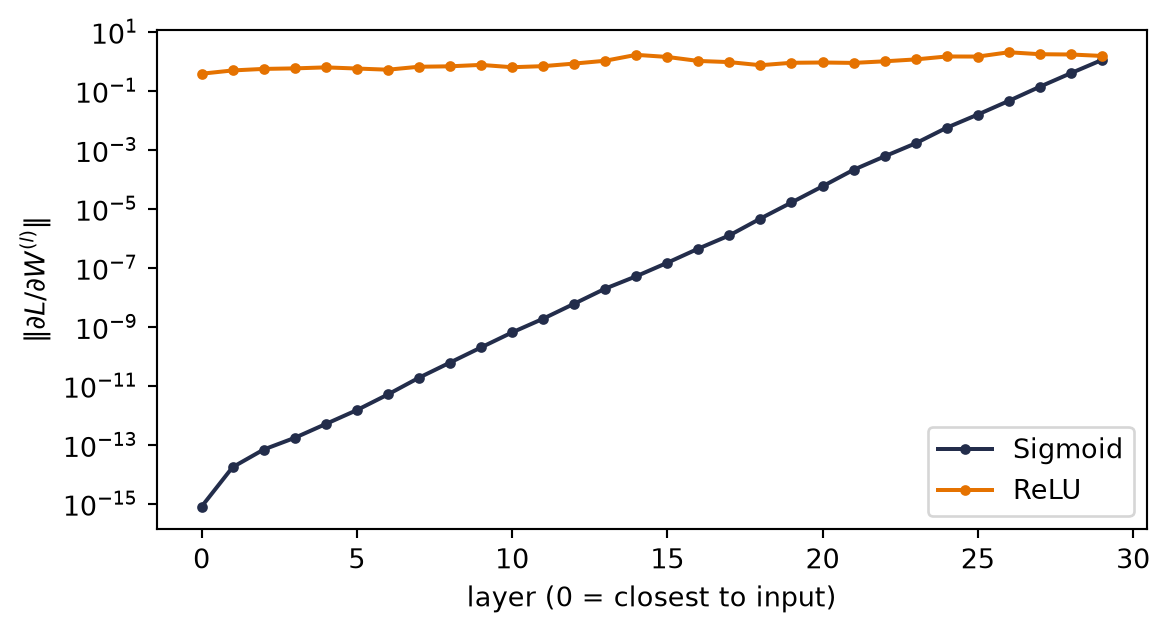

Figure 5.6: Gradient reaching each layer of two matched 30-layer MLPs (float64 norm, log scale). With the same He-scaled weights and inputs, repeated sigmoid derivatives leave a nonzero but unusably small first-layer signal; ReLU preserves enough signal for a float32 update to change every first-layer weight.

Sigmoid: max|g0|=9.47e-17; nonzero=4096/4096; changed=0/4096
ReLU   : max|g0|=2.54e-02; nonzero=4096/4096; changed=4096/4096

Read the slopes, then read the printed counts of nonzero gradient entries and changed weights. All 4,096 sigmoid first-layer entries survive the float32 cast as nonzero numbers. They are so small, however, that subtracting \(0.1g\) changes none of the stored float32 weights. The ReLU network changes all 4,096. That distinction matters, and Appendix C names both failures: a displayed float32 norm can underflow while individual entries remain nonzero, and a nonzero entry can still produce an update that rounds away when subtracted from a larger stored weight.

5.7 Initialization and signal scale

The weights also scale the signal at each layer, so their initial scale is a second factor we choose. If each layer multiplies the variance of the signal by more than one, activations explode after enough layers; by less than one, they vanish, and by Equation 5.3 the gradients follow. A good initialization keeps the variance roughly constant in both directions.

The variance scales predictably through the dot product. For \(z = \sum_{i=1}^{n_{\text{in}}} w_i x_i\) with independent, zero-mean inputs and weights, \(\var(z) = n_{\text{in}} \var(w) \var(x)\). Keeping \(\var(z) = \var(x)\) demands the first condition below. On the backward pass, each input unit collects a sum over the units it fed, so keeping the variance of the sensitivities constant demands the second:

\[ \var(w) = \frac{1}{n_{\text{in}}} \quad \text{(forward)}, \qquad \var(w) = \frac{1}{n_{\text{out}}} \quad \text{(backward)}. \]

Xavier initialization balances the forward and backward variance criteria, \(\var(w) = 2/(n_{\text{in}} + n_{\text{out}})\). He initialization accounts for ReLU discarding half its input distribution by doubling the forward recipe, \(\var(w) = 2/n_{\text{in}}\). A PyTorch linear layer follows neither recipe by default: it draws its weights uniformly with variance \(1/(3n_{\text{in}})\), a sixth of the He value \(2/n_{\text{in}}\), so a deep ReLU stack without normalization needs an explicit choice.

1. Define the reusable signal_std helper.
2. Fix the seed, define two naive weight scales (0.05, 0.12) and He scaling, and open the figure.
3. Signal energy vs depth.
4. Add a legend naming each initialization scheme and show the plot.

from collections.abc import Callable

# [1]
def signal_std(
    scale_fn: Callable[[torch.Tensor, int], torch.Tensor],
    depth: int = 40, width: int = 256
) -> list[float]:
    x = torch.randn(512, width)
    stds = []
    for _ in range(depth):
        W = scale_fn(torch.randn(width, width), width)
        x = torch.relu(x @ W)
        stds.append(x.std().item())
    return stds

# [2]
torch.manual_seed(6050)
schemes = {
    "naive  (std = 0.05)": lambda W, n: W * 0.05,
    "naive  (std = 0.12)": lambda W, n: W * 0.12,
    "He  (std = sqrt(2/n))": lambda W, n: W * (2 / n) ** 0.5,
}
plt.figure(figsize=(6.2, 3.4))
# [3]
for (name, fn), color in zip(schemes.items(), ["#5379AA", "#722F37", "#E57200"]):
    plt.semilogy(signal_std(fn), color=color, label=name)
plt.xlabel("layer"); plt.ylabel("std of activations")
# [4]
plt.legend(); plt.tight_layout(); plt.show()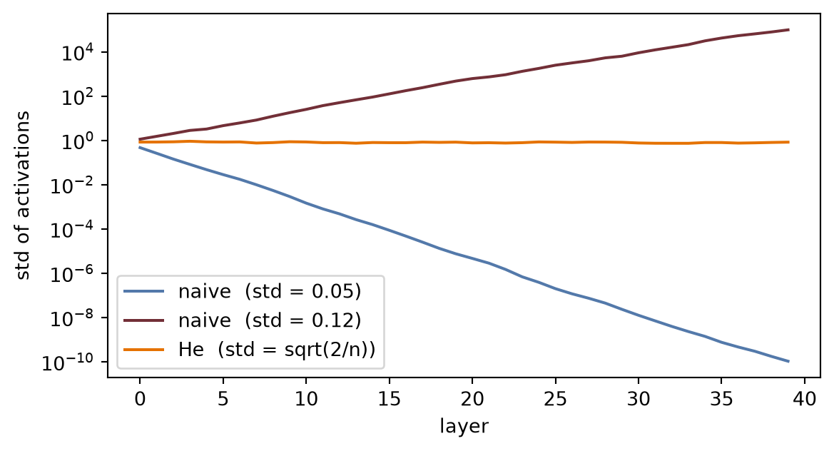

Figure 5.7: Activation standard deviation through 40 ReLU layers of width \(n = 256\). Each fixed weight scale multiplies the signal by a roughly constant factor per layer, a straight line on the log axis; the He-initialized trace stays near its starting scale in this run.

Over 40 layers, the two fixed scales, \(0.05\) and \(0.12\), move the signal by many orders of magnitude before training starts, while the He scale keeps it level. Initialization sets the starting scale of the weights, and the choice of activation determines the derivative factors; together they decide whether the forward and backward signals survive depth at the start of training. Two later tools work on the same problem during training: normalization layers rescale intermediate computations, and skip connections add paths that bypass a block’s activation derivatives and weights alike. Normalization and the residual idea arrive in Chapter 10, and layer normalization becomes essential inside the Transformer of Chapter 16.

NoteCheck yourself

Close the book for one minute and run the chain rule backward.

• What does each layer cache on the forward pass, and what does that cost in memory?
• Why does the sensitivity \(\delta\) pass through a transposed weight matrix?
• How do activation derivatives and initialization together control gradient scale with depth?

5.8 Okay, so: the chain rule, organized

1. The graph. Any network is a computation graph; the forward pass computes and caches, while the backward pass multiplies local derivatives in reverse and sums contributions from multiple paths.
2. The sensitivity. \(\delta^{(l)} = \partial L / \partial \vect{z}^{(l)}\) turns the tangle into four equations: start at the output (Equation 5.2), propagate through \(\matr{W}^\top\) and the activation derivative (Equation 5.3), then read off weight and bias gradients (Equation 5.4, Equation 5.5). On a batch, each forward matrix product costs two backward ones, so the sweep delivers every gradient for about twice the forward arithmetic, paid for in cached activations.
3. We verified it: our hand-built equations match PyTorch’s autograd to \(10^{-8}\). The scalar engine illustrates reverse topological order and adjoint accumulation by addition.
4. Activation derivatives and depth. The sigmoid-derivative product along a path is bounded above by \(0.25^k\) after \(k\) activation-derivative factors. ReLU has an activation derivative of one on positive inputs. Initialization helps control activation and gradient scales at the start of training.

Backpropagation trains every model from here through Chapter 23. The next time a deep model fails to learn, your first questions now have names: is the gradient reaching the early layers? what is attenuating it? what is its scale?

Sources and further reading

• Rumelhart, Hinton, and Williams, “Learning representations by back-propagating errors” (1986): the landmark short account of learning internal representations by reverse error propagation.
• Baydin et al., “Automatic Differentiation in Machine Learning: a Survey” (2018): separates reverse-mode automatic differentiation from symbolic and numerical differentiation.
• Glorot and Bengio, “Understanding the difficulty of training deep feedforward neural networks” (2010): the variance argument behind Xavier initialization.
• He et al., “Delving Deep into Rectifiers” (2015): derives the rectifier-aware initialization used in the matched depth experiment.
• CS231n, “Gradient Checks”: the centered-difference and relative-error safeguards used in Exercise 6.
• Chen, Xu, Zhang, and Guestrin, “Training Deep Nets with Sublinear Memory Cost” (2016): stores a subset of activations and recomputes the rest during the backward pass, trading arithmetic for memory.
• Shakeri, Deep Learning: Making It Trainable, Chapter 11, “The Gradient Has a Memory: Reverse Accumulation and Checkpointing” (2026): a treatment of reverse accumulation as a memory and numerical diagnostic, including fan-out accumulation, vector–Jacobian products, retained state, and checkpoint replay.

Exercises

1. (Pencil.) Derive the four layer equations for a network whose output layer uses the identity activation and squared-error loss (the network of our verification cell). Confirm that your \(\delta^{(2)}\) matches the one that cell computes.
2. (Pencil.) In Equation 5.3, why does the sensitivity pass through \((\matr{W}^{(l+1)})^\top\) rather than \(\matr{W}^{(l+1)}\)? Argue from shapes: what are the dimensions of \(\delta^{(l)}\), \(\delta^{(l+1)}\), and \(\matr{W}^{(l+1)}\)? Then check that the batched form \(\bigl(\matr{\Delta}^{(2)}\matr{W}^{(2)}\bigr) \odot \sigma'(\matr{Z}^{(1)})\) in our verification cell has consistent shapes too.
3. (Code.) Extend the Value class with tanh and use it to train the one-neuron model from the check cell for 50 steps (write the update loop yourself). Verify the loss decreases.
4. (Code.) In the depth experiment, give the sigmoid network Xavier initialization (nn.init.xavier_normal_ on each linear layer). How much of the vanishing does good initialization recover at depth 30? What does that tell you about why both fixes, initialization and ReLU, became standard?
5. (Code.) Comment out optimizer.zero_grad() in any training loop from Chapter 1 and describe what happens to the loss curve. Explain it with one sentence about gradient accumulation.
6. (Pencil.) Derive why a forward finite difference has truncation error \(O(\varepsilon)\) while a centered difference has error \(O(\varepsilon^2)\). (Audit.) Gradient-check this chapter’s two-layer manual backward pass with \(|g_a-g_n|/\max(10^{-12},|g_a|,|g_n|)\) for \(\varepsilon=10^{-2},\ldots,10^{-10}\) in float32 and float64. Plot relative error, explain its U-shape as truncation meets rounding, and require agreement across several randomly selected parameters under a fixed seed. Named wrong answer: “absolute error below \(10^{-4}\) proves the gradient”: absolute error ignores the scale of the quantity being checked.
7. (Pencil.) Let \(\hat{\vect{y}} = \operatorname{softmax}(\vect{o})\) for logits \(\vect{o} \in \mathbb{R}^K\). Show that its Jacobian is \(\partial\hat{\vect{y}}/\partial\vect{o} = \operatorname{diag}(\hat{\vect{y}}) - \hat{\vect{y}}\hat{\vect{y}}^\top\), and that for any upstream sensitivity \(\vect{u} = \partial L/\partial\hat{\vect{y}}\) the vector–Jacobian product is \(\partial L/\partial\vect{o} = \hat{\vect{y}} \odot \bigl(\vect{u} - \langle\vect{u}, \hat{\vect{y}}\rangle\,\mathbf{1}\bigr)\), which costs \(O(K)\) where forming the Jacobian costs \(O(K^2)\). Choose \(\vect{u}\) for \(L = -\log \hat{y}_c\) and recover Equation 2.6; choose it for squared error against a one-hot target and recover the row formula in Exercise 4 of Chapter 2. (Code.) Implement softmax_vjp(y_hat, u), check it against torch.autograd.grad in float64 for random logits and upstream vectors under a fixed seed, and time it against multiplying by the materialized Jacobian for \(K = 10^2, 10^3, 10^4\).