20  Adapting Pretrained Models: Prompting, PEFT, Quantization

Chapter tools Lecture slides 11.1 · ICL, Prompt Engineering, and RAG·Lecture slides 11.2 · Parameter-Efficient Fine-Tuning·Lecture slides 11.3 · Quantization and QLoRA·Download notebook·Open in Colab (opens in a new tab)

Chapter 10 compared training from scratch with adapting a pretrained representation. We now examine the resource costs of that adaptation. Changing the input context, restricting parameter updates, and reducing numerical precision modify different parts of the computation. Their usefulness must be evaluated on the target task.

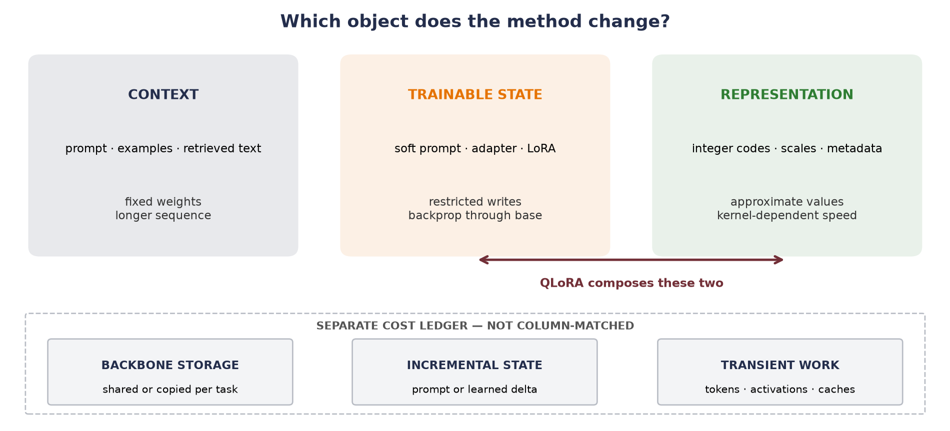
Reusing a pretrained model has three different costs:

1. the backbone storage: a base shared across tasks, or a full task-specific copy when sharing is abandoned;
2. the incremental task state: the prompt, adapter, or unmerged delta that makes one task different from another; and
3. the transient work: context tokens, activations, gradients, optimizer state, and caches needed while adapting or running the model.

These costs are related, but they are not interchangeable: every lever can affect more than one cost, and none removes all backbone storage or transient work. Freezing a billion weights removes their gradients; it does not make the billion weights disappear. Packing each weight into fewer bits reduces a storage lower bound; it does not prove that a particular kernel will run faster. Adding demonstrations changes no weight; it still lengthens the sequence the model must process. A merged LoRA or fully tuned checkpoint can collapse base and delta into one artifact, but then each task carries a full backbone-sized copy instead of sharing the original.

So we ask not simply “How many parameters?” but where does task-specific information live, and which object does the method change? Hard prompts and retrieved documents place task information in context. Parameter-efficient fine-tuning (PEFT) places it in a restricted set of learned values. Quantization need not add task information at all; it changes the numerical representation of a base or adapter. QLoRA composes the last two.

Figure 20.1: Three levers act on three different objects. Prompting changes the context presented to a fixed model; PEFT lets only a small learned state receive gradient updates; quantization changes how fixed values are represented. QLoRA combines a quantized frozen base with a trainable low-rank branch. The dashed row of costs below is deliberately not aligned with the columns above: each lever can affect several costs.

20.1 Prompting: move evidence into context

A decoder in Chapter 16 already defines a conditional distribution over the next token. Prompting changes the prefix on which that fixed distribution is conditioned. For an instruction \(I\), demonstrations \((x_i,y_i)\), and a query \(x_\star\), a discrete prompted prediction can be written

\[ \hat y =\argmax_y p_{\theta_0}\!\left( y\mid I,(x_1,y_1),\ldots,(x_k,y_k),x_\star \right), \qquad \theta_{\text{after}}=\theta_{\text{before}}=\theta_0. \tag{20.1}\]

The weights never move; only the context does. With no demonstrations, this is zero-shot prompting. With a few, it is few-shot prompting; when the model uses those examples to infer the task inside its forward computation, we call the behavior in-context learning (ICL). The word learning means that behavior changes with the context, not that a checkpoint is updated.

Brown and colleagues found that few-shot gains often grew with model scale in GPT-3, but that is an empirical result over particular models and tasks. It does not establish universal parameter thresholds, nor does it settle the mechanism by which a Transformer uses demonstrations. Attention lets later positions see earlier examples and route information from them; saying it literally “performs analogy” would outrun the evidence. Prompt order, label words, formatting, and example choice can all matter. Controlled ablations have found that demonstration inputs, the label space and its mapping, formatting, and ordering can contribute differently across tasks. Those results constrain simple stories about copying examples, but they do not settle one universal causal mechanism for ICL.

Instructions that ask for intermediate steps can improve some multi-step tasks. Those visible steps are generated tokens, however, not a guaranteed faithful window into the model’s internal computation. The same logits and decoding cautions from Chapter 13 still apply.

NotePrompting is not prompt tuning

A hard prompt is a sequence of ordinary token IDs chosen by a person or program. It receives no gradient. Prompt tuning, introduced later in this chapter, learns continuous vectors by backpropagation and is therefore a PEFT method. Similar names do not mean the same training procedure.

Zero trainable parameters is not zero cost: demonstrations consume context length. They increase prefill work, the initial forward pass that processes the supplied prefix, and occupy entries in the key/value (KV) cache, the stored attention keys and values reused while autoregressively generating later tokens. They also expose task data at inference time. Prompting trades a new checkpoint for a longer, more carefully constructed input.

A frozen-context mechanism test

Can a fixed network genuinely change its answer because examples in the prompt reveal a task? We can test that mechanism without claiming to reproduce natural-language ICL.

Each synthetic episode assigns four group symbols to four label symbols by a hidden permutation. A demonstration reveals one group–label pair; demo groups are distinct. A two-shot prompt might read [BOS] group C, label A; group A, label D; [QUERY] group A, whose target is label D. The query names one group, demonstrated or not, and asks for its label. We meta-train a tiny causal Transformer across many such episodes, cycling through one to four demonstrations. During evaluation, it receives a new random mapping and no parameter update.

The information ceiling is known before training. With \(k<4\) demonstrations, the query group, drawn uniformly from the four groups, already appears among them with probability \(k/4\). Otherwise, its label is uniform among the \(4-k\) unused labels. Therefore

\[ \Pr(\text{correct}\mid k) = \begin{cases} \dfrac{k}{4}+\left(1-\dfrac{k}{4}\right)\dfrac{1}{4-k} =\dfrac{k+1}{4}, & 0\le k\le3,\\[6pt] 1, & k=4. \end{cases} \tag{20.2}\]

At \(k=3\), even an unseen query group is solvable by elimination. Accuracy on such queries will tell us whether the model merely copies a seen pair or uses the whole mapping.

The code uses nn.TransformerEncoderLayer as a compact container for the same pre-LayerNorm attention–residual–FFN structural pattern built from first principles in Chapter 16. Its GELU choice differs from that chapter’s teaching block; the wrapper does not hide the causal or padding masks, embeddings, or classifier. Token IDs have shape \([B,11]\), hidden states \([B,11,48]\), and the query logits \([B,4]\).

1. Fix the special token IDs, the group and label offsets, 11 vocabulary tokens, 11 positions, and four classes.
2. Define the reusable helpers: sample_episode_bank, render_episodes, and ContextLearner.
3. Define the reusable helpers: evaluate_context and run_context_seed.
4. Meta-train a tiny causal Transformer, then audit frozen-weight in-context adaptation over five seeds.

# [1]
PAD, BOS, QUERY = 0, 1, 2
GROUP0, LABEL0 = 3, 7
VOCAB, SEQUENCE_LENGTH, N_CLASSES = 11, 11, 4


# [2]
def sample_episode_bank(
    batch_size: int, generator: torch.Generator
) -> tuple[torch.Tensor, torch.Tensor, torch.Tensor]:
    mapping = torch.rand(batch_size, N_CLASSES, generator=generator).argsort(dim=1)
    demo_groups = torch.rand(
        batch_size, N_CLASSES, generator=generator
    ).argsort(dim=1)
    query_groups = torch.randint(
        N_CLASSES, (batch_size,), generator=generator
    )
    return mapping, demo_groups, query_groups


def render_episodes(
    bank: tuple[torch.Tensor, torch.Tensor, torch.Tensor], k: int
) -> tuple[torch.Tensor, torch.Tensor, torch.Tensor]:
    mapping, demo_groups, query_groups = bank
    tokens = torch.full((len(mapping), SEQUENCE_LENGTH), PAD, dtype=torch.long)
    tokens[:, 0] = BOS
    for slot in range(k):
        group = demo_groups[:, slot]
        label = mapping.gather(1, group[:, None]).squeeze(1)
        tokens[:, 1 + 2 * slot] = GROUP0 + group
        tokens[:, 2 + 2 * slot] = LABEL0 + label
    tokens[:, 9] = QUERY
    tokens[:, 10] = GROUP0 + query_groups
    targets = mapping.gather(1, query_groups[:, None]).squeeze(1)
    covered = (
        (demo_groups[:, :k] == query_groups[:, None]).any(dim=1)
        if k else torch.zeros(len(mapping), dtype=torch.bool)
    )
    return tokens, targets, covered


class ContextLearner(nn.Module):
    def __init__(self, width: int = 48, heads: int = 4, layers: int = 2) -> None:
        super().__init__()
        self.token = nn.Embedding(VOCAB, width, padding_idx=PAD)
        self.position = nn.Embedding(SEQUENCE_LENGTH, width)
        layer = nn.TransformerEncoderLayer(
            d_model=width, nhead=heads, dim_feedforward=2 * width,
            dropout=0.0, batch_first=True, norm_first=True, activation="gelu",
        )
        self.encoder = nn.TransformerEncoder(
            layer, layers, norm=nn.LayerNorm(width), enable_nested_tensor=False
        )
        self.head = nn.Linear(width, N_CLASSES)
        self.register_buffer(
            "causal",
            torch.triu(torch.ones(SEQUENCE_LENGTH, SEQUENCE_LENGTH, dtype=torch.bool),
                       diagonal=1),
        )

    def forward(self, tokens: torch.Tensor) -> torch.Tensor:
        positions = torch.arange(SEQUENCE_LENGTH, device=tokens.device)
        hidden = self.token(tokens) + self.position(positions)[None]
        hidden = self.encoder(
            hidden, mask=self.causal, src_key_padding_mask=tokens.eq(PAD)
        )
        return self.head(hidden[:, -1])


# [3]
@torch.no_grad()
def evaluate_context(
    model: nn.Module, seed: int, n: int = 8192
) -> tuple[list[dict], bool]:
    model.eval()
    before = [parameter.detach().clone() for parameter in model.parameters()]
    bank = sample_episode_bank(n, torch.Generator().manual_seed(seed + 10_000))
    rows = []
    for k in range(5):
        tokens, targets, covered = render_episodes(bank, k)
        correct = model(tokens).argmax(1).eq(targets)
        rows.append({
            "k": k,
            "accuracy": correct.float().mean().item(),
            "covered": correct[covered].float().mean().item()
                       if covered.any() else float("nan"),
            "uncovered": correct[~covered].float().mean().item()
                         if (~covered).any() else float("nan"),
        })
    unchanged = all(
        torch.equal(old, new) for old, new in zip(before, model.parameters())
    )
    return rows, unchanged


def run_context_seed(seed: int, steps: int = 1200) -> dict:
    torch.manual_seed(seed)
    generator = torch.Generator().manual_seed(seed)
    model = ContextLearner()
    optimizer = torch.optim.AdamW(model.parameters(), lr=3e-3, weight_decay=1e-2)
    scheduler = torch.optim.lr_scheduler.CosineAnnealingLR(
        optimizer, T_max=steps, eta_min=3e-5
    )
    model.train()
    for step in range(steps):
        k = 1 + step % 4
        bank = sample_episode_bank(256, generator)
        tokens, targets, _ = render_episodes(bank, k)
        loss = F.cross_entropy(model(tokens), targets)
        optimizer.zero_grad(set_to_none=True)
        loss.backward()
        nn.utils.clip_grad_norm_(model.parameters(), 1.0)
        optimizer.step()
        scheduler.step()
    rows, unchanged = evaluate_context(model, seed)
    return {
        "seed": seed,
        "rows": rows,
        "unchanged": unchanged,
        "parameters": sum(parameter.numel() for parameter in model.parameters()),
    }


CONTEXT_SEEDS = list(range(6050, 6055))
context_runs = [run_context_seed(seed) for seed in CONTEXT_SEEDS]
context_accuracy = np.array([
    [row["accuracy"] for row in run["rows"]] for run in context_runs
])
context_ceiling = np.array([0.25, 0.50, 0.75, 1.00, 1.00])

print("model parameters:", f'{context_runs[0]["parameters"]:,}')
print("k  mean accuracy  seed sd  information ceiling")
# [4]
for k in range(5):
    print(
        f"{k}      {context_accuracy[:, k].mean():.3f}       "
        f"{context_accuracy[:, k].std(ddof=1):.3f}          "
        f"{context_ceiling[k]:.2f}"
    )
print("all evaluation passes left weights unchanged:",
      all(run["unchanged"] for run in context_runs))

model parameters: 39,268
k  mean accuracy  seed sd  information ceiling
0      0.252       0.003          0.25
1      0.500       0.005          0.50
2      0.749       0.002          0.75
3      1.000       0.000          1.00
4      1.000       0.000          1.00
all evaluation passes left weights unchanged: True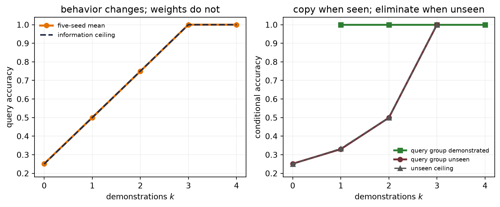

Figure 20.2: A frozen model changes behavior as demonstrations reveal an episode’s hidden label mapping. Across five independently trained seeds, overall accuracy (left) closely tracks the analytical information ceiling. Conditional accuracy (right) is perfect when the query group appeared; for unseen groups it follows the shrinking set of unused labels and reaches 1 at three demonstrations by elimination. Evaluation uses one nested episode bank per seed, and every parameter is bitwise unchanged across all five context lengths.

The 39,268-parameter network lands at mean accuracies \(0.252,0.500,0.749,1.000,1.000\) for \(k=0,1,2,3,4\), respectively. The analytic ceilings are \(0.25,0.50,0.75,1,1\). More revealingly, unseen-query accuracy rises from \(0.252\) to \(0.330\), \(0.499\), and \(1.000\). The model is not only copying a matching demonstration; at \(k=3\) it identifies the remaining label.

WarningAn existence proof in a designed regime

The model was meta-trained on exactly this family of random permutation tasks. The study demonstrates that a frozen causal Transformer can use prompt evidence in this controlled distribution. It does not estimate natural-language ICL quality, explain the mechanism inside a large language model, or show that more examples always help. From one run to the next, the initialization, the meta-training episodes, and the finite 8,192-episode evaluation bank all change. The seed SD therefore measures combined run-to-run repeatability, not task or domain diversity, and not optimization alone.

Retrieval is another context lever

A prompt can contain information selected at query time rather than written by hand. Retrieval-augmented generation (RAG) first searches an external corpus, then places retrieved passages beside the instruction and query before generation. The generator’s weights may remain fixed; the task-specific state lives partly in the index and partly in the retrieved context.

As in Chapter 14, a retriever computes query–document similarities, selects neighbors, and hands their content to a downstream weighted computation. Modern systems can learn the retriever, the generator, or both, but the basic context-augmentation move is distinct from PEFT.

Retrieval moves rather than abolishes failure: a missed document cannot support the answer; a highly ranked irrelevant passage can distract it; retrieved text can contain malicious instructions; and a plausible citation does not prove that the generated claim follows from the cited evidence. RAG is attractive when facts change faster than checkpoints or when provenance matters, but it is a pipeline whose retrieval and generation stages must be evaluated separately.

20.2 What if the prompt itself were learnable?

Hard prompts spend human effort and context tokens. What if the prompt itself were learnable? Let \(\matr{P}\in\mathbb{R}^{m\times d}\) be \(m\) continuous vectors with the same width as token embeddings. For an \(n\)-token input, define \(\operatorname{Embed}(x)\in\mathbb{R}^{n\times d}\). Prompt tuning prepends the learned rows,

\[ \matr{H}^{(0)}=[\matr{P};\operatorname{Embed}(x)], \qquad \min_{\matr{P}} -\sum_i\log p_{\theta_0,\matr{P}}(y_i\mid x_i), \tag{20.3}\]

while freezing \(\theta_0\). Not counting any task head, the learned state contains exactly \(md\) values. Those values are not words, and need not be nearest to any vocabulary embedding. They are virtual tokens optimized by gradient descent, and they still occupy \(m\) virtual sequence positions during use.

Prefix tuning moves a related idea deeper. At every Transformer layer \(\ell\), let the ordinary keys and values be \(\matr{K}_\ell,\matr{V}_\ell\in\mathbb{R}^{n\times d}\) and the learned prefixes be \(\matr{P}^K_\ell,\matr{P}^V_\ell\in\mathbb{R}^{m\times d}\). The prefix rows extend the ordinary keys and values:

\[ \matr{K}'_\ell=[\matr{P}^K_\ell;\matr{K}_\ell], \qquad \matr{V}'_\ell=[\matr{P}^V_\ell;\matr{V}_\ell]. \]

A direct implementation with \(m\) prefix slots, width \(d\), and \(L\) layers stores \(2Lmd\) values, although practical parameterizations can differ. Li and Liang used an auxiliary network during optimization, then retained only the learned prefix for inference. Lester and colleagues found that prompt tuning approached full tuning as T5 scale grew in their SuperGLUE study; that result is not a universal size threshold.

Two other PEFT families act inside frozen blocks. Adapters insert a small bottleneck inside each frozen Transformer block. For bottleneck width \(d_b\), let \(\matr{W}_{\mathrm{down}}\in\mathbb{R}^{d_b\times d}\), \(\vect{b}_{\mathrm{down}}\in\mathbb{R}^{d_b}\), \(\matr{W}_{\mathrm{up}}\in\mathbb{R}^{d\times d_b}\), and \(\vect{b}_{\mathrm{up}}\in\mathbb{R}^{d}\). One common residual form is

\[ \operatorname{Adapter}(\vect{h}) =\vect{h} +\matr{W}_{\mathrm{up}} \sigma(\matr{W}_{\mathrm{down}}\vect{h}+\vect{b}_{\mathrm{down}}) +\vect{b}_{\mathrm{up}}. \]

This module adds \(2dd_b+d+d_b\) parameters. BitFit takes the selective-update idea to an extreme: freeze pretrained weight matrices and update their existing bias terms. The original BitFit classification experiments also trained the task-specific output layer; “bias-only” describes the restriction inside the pretrained backbone. Neither method promises the same accuracy on every task. They are different restrictions on where gradient updates may write.

20.3 LoRA: a low-rank correction beside a frozen path

Consider one frozen linear map

\[ \matr{W}_0\in\mathbb{R}^{d_{\mathrm{out}}\times d_{\mathrm{in}}}, \qquad \vect{h}=\matr{W}_0\vect{x}. \]

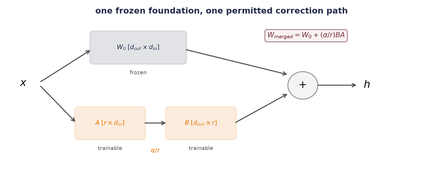
Full fine-tuning learns an unrestricted correction \(\Delta\matr{W}\) with \(d_{\mathrm{out}}d_{\mathrm{in}}\) values. Low-Rank Adaptation (LoRA) instead constrains the correction to a product of two thin matrices:

\[ \Delta\matr{W} =\frac{\alpha}{r}\matr{B}\matr{A}, \qquad \matr{A}\in\mathbb{R}^{r\times d_{\mathrm{in}}}, \quad \matr{B}\in\mathbb{R}^{d_{\mathrm{out}}\times r}. \tag{20.4}\]

The forward pass is

\[ \vect{h} =\matr{W}_0\vect{x} +\frac{\alpha}{r}\matr{B}(\matr{A}\vect{x}). \tag{20.5}\]

\(\matr{A}\) compresses to \(r\) coordinates and \(\matr{B}\) expands back to the output width. Because \(\operatorname{rank}(\matr{B}\matr{A})\le r\), task updates can use at most \(r\) independent linear directions in that matrix. Only the correction is constrained to rank at most \(r\). The merged matrix need not be low rank.

The trainable count is

\[ P_{\mathrm{LoRA}} =r(d_{\mathrm{in}}+d_{\mathrm{out}}). \tag{20.6}\]

For one \(4096\times4096\) map and \(r=16\), full tuning exposes 16,777,216 values; LoRA exposes \(16(4096+4096)=131{,}072\), or \(0.78125\%\). A model-level percentage requires summing Equation 20.6 over the matrices actually targeted. The original LoRA experiments emphasized query and value projections; later recipes often target different or more numerous matrices. “Rank 16” alone does not specify an adapter’s size.

TipPractice bridge (optional): read PEFT through a library’s algebra

A PEFT library expresses Equation 20.4 through a package wrapper. Treat the wrapper’s names as a translation layer, not as new mathematics:

• r is the inner dimension of \(A\) and \(B\);
• lora_alpha / r represents the factor \(\alpha/r\);
• target_modules chooses which frozen maps play the role of \(W_0\);
• the adapter checkpoint carries the learned factors, while the base checkpoint supplies the frozen path.

If the wrapper targets “all linear” modules, do not infer the adapter size from that phrase. Inspect the selected module names and shapes, sum Equation 20.6 over exactly that set, and print the parameters that still have requires_grad=True. Then apply the four-part freeze audit below: the base stays unchanged, only permitted factors receive gradients, and merged and unmerged outputs agree within a declared numerical tolerance. Package calls and model identifiers can evolve; these algebraic checks do not.

When the base is also stored on a quantization grid, the result is QLoRA, not a different LoRA equation. Keep the frozen base’s storage and compute dtypes separate from the factors’ trainable dtype, as Appendix C requires. The QLoRA section later in this chapter makes that composition explicit.

Figure 20.3: LoRA adds a trainable low-rank branch beside a frozen linear map. The gradient flows through both computational paths, but only A and B receive updates. Initializing A randomly and B to zero begins with an exact zero correction while leaving a nonzero first gradient for B; after training, the correction can be merged into a compatible base weight.

The usual initialization samples \(\matr{A}\) and sets \(\matr{B}=0\). The initial correction is then exactly zero, yet \(\matr{B}\) can receive a gradient because \(\matr{A}\vect{x}\) is generally nonzero. Setting both factors to zero would block both first gradients. The scale \(\alpha/r\) separates a chosen adapter strength from rank, but its best value remains a tuning decision.

Once trained, a single compatible adapter can be merged:

\[ \matr{W}_{\mathrm{merged}} =\matr{W}_0+\frac{\alpha}{r}\matr{B}\matr{A}. \tag{20.7}\]

Merged and unmerged arithmetic should agree to numerical tolerance. Only the merged form removes the extra branch at inference. Dynamic adapter switching, keeping many adapters active, or combining LoRA with a quantized base changes whether and how we merge; a quantized merge generally requires dequantization and requantization.

TipA four-part freeze audit

Count trainable values; assert the base tensor is bitwise unchanged; check that only permitted parameters receive gradients; and compare merged with unmerged outputs. A small checkpoint is not evidence that the intended tensors were frozen. The assertions belong beside the implementation, not in a comment after training.

Make the rank bottleneck fail on purpose

Low rank is a hypothesis about the update, not a free compression theorem. We can make its boundary visible by planting a target correction with exactly six independent diagonal directions. The frozen base is a \(32\times32\) map. Full tuning may move all 1,024 entries; LoRA may use ranks \(1,2,4,6,\) or \(8\). Inputs are fixed Gaussian vectors, targets are noiseless, and five LoRA initializations see the same problem and optimizer schedule.

Write the six planted magnitudes as \(\sigma_1\ge\cdots\ge\sigma_6\). Their values are \(1.20,0.90,0.65,0.40,0.22,0.10\). A correction whose rank \(r\) is below six must leave some directions behind. Because the target is exactly low rank, we can compute the error each rank must leave before we train.

Because the six diagonal basis directions are mutually orthogonal, their squared correction energy is \(\sum_{j=1}^{6}\sigma_j^2\). A rank-\(r\) correction can retain at most \(r\) independent directions. The planted correction is diagonal with positive entries, so \(\sigma_1,\ldots,\sigma_6\) are its nonzero singular values. By the Eckart–Young–Mirsky result, Equation A.10 in Appendix A, no correction of rank at most \(r\) is closer to the planted correction in Frobenius norm than the truncation that keeps its \(r\) largest magnitudes. That truncation leaves the concrete relative floor

\[ \epsilon_r =\sqrt{\frac{\sum_{j=r+1}^{6}\sigma_j^2} {\sum_{j=1}^{6}\sigma_j^2}}, \qquad r<6, \tag{20.8}\]

and zero for \(r\ge6\). The plotted “capacity floor” is this calculation, not a result estimated from the optimizer.

1. Fix the 32×32 layer shape, the target rank of six, and the six direction magnitudes.
2. Define the reusable helpers: make_rank_problem, FullUpdate, and LoRAUpdate.
3. Define the reusable helpers: train_linear_update and relative_update_error.
4. Compare frozen, full, and low-rank updates against a planted rank-six correction.
5. Check the claimed identities, shapes, or invariants.
6. Print frozen and full-update errors, a per-rank table of seed means, and the largest merged/unmerged gap.

# [1]
D_IN = D_OUT = 32
TARGET_RANK = 6
DIRECTION_MAGNITUDES = torch.tensor([1.20, 0.90, 0.65, 0.40, 0.22, 0.10])


# [2]
def make_rank_problem(
    seed: int = 1700,
) -> tuple[torch.Tensor, torch.Tensor, torch.Tensor, torch.Tensor,
           torch.Tensor, torch.Tensor]:
    generator = torch.Generator().manual_seed(seed)
    base = torch.randn(D_OUT, D_IN, generator=generator) / math.sqrt(D_IN)
    correction = torch.zeros(D_OUT, D_IN)
    diagonal = torch.arange(TARGET_RANK)
    correction[diagonal, diagonal] = DIRECTION_MAGNITUDES
    x_train = torch.randn(1024, D_IN, generator=generator)
    x_validation = torch.randn(4096, D_IN, generator=generator)
    y_train = F.linear(x_train, base + correction)
    y_validation = F.linear(x_validation, base + correction)
    return base, correction, x_train, y_train, x_validation, y_validation


class FullUpdate(nn.Module):
    def __init__(self, base: torch.Tensor) -> None:
        super().__init__()
        self.weight = nn.Parameter(base.clone())

    def forward(self, x: torch.Tensor) -> torch.Tensor:
        return F.linear(x, self.weight)


class LoRAUpdate(nn.Module):
    def __init__(
        self, base: torch.Tensor, rank: int, generator: torch.Generator
    ) -> None:
        super().__init__()
        self.register_buffer("weight0", base.clone())
        self.A = nn.Parameter(torch.randn(rank, D_IN, generator=generator) * 0.02)
        self.B = nn.Parameter(torch.zeros(D_OUT, rank))
        self.rank = rank
        self.alpha = rank

    @property
    def scaling(self) -> float:
        return self.alpha / self.rank

    def forward(self, x: torch.Tensor) -> torch.Tensor:
        low_rank = F.linear(F.linear(x, self.A), self.B)
        return F.linear(x, self.weight0) + self.scaling * low_rank

    def merged_weight(self) -> torch.Tensor:
        return self.weight0 + self.scaling * (self.B @ self.A)


# [3]
def train_linear_update(
    model: nn.Module, x: torch.Tensor, y: torch.Tensor, steps: int = 1200
) -> None:
    optimizer = torch.optim.Adam(model.parameters(), lr=0.03)
    scheduler = torch.optim.lr_scheduler.CosineAnnealingLR(
        optimizer, T_max=steps, eta_min=3e-4
    )
    for _ in range(steps):
        loss = F.mse_loss(model(x), y)
        optimizer.zero_grad(set_to_none=True)
        loss.backward()
        optimizer.step()
        scheduler.step()


def relative_update_error(
    estimate: torch.Tensor, target: torch.Tensor
) -> float:
    return (torch.linalg.norm(estimate - target) / torch.linalg.norm(target)).item()


base, target_delta, x_train, y_train, x_val, y_val = make_rank_problem()
target_energy = torch.sum(DIRECTION_MAGNITUDES ** 2)

full_model = FullUpdate(base)
# [4]
train_linear_update(full_model, x_train, y_train)
with torch.no_grad():
    full_mse = F.mse_loss(full_model(x_val), y_val).item()
    full_relative_error = relative_update_error(
        full_model.weight - base, target_delta
    )
    frozen_mse = F.mse_loss(F.linear(x_val, base), y_val).item()

LORA_RANKS = [1, 2, 4, 6, 8]
lora_runs = []
# [5]
for seed in range(6050, 6055):
    for rank in LORA_RANKS:
        model = LoRAUpdate(
            base, rank, torch.Generator().manual_seed(seed + rank)
        )
        frozen_before = model.weight0.clone()
        train_linear_update(model, x_train, y_train)
        with torch.no_grad():
            merged = model.merged_weight()
            merge_error = (
                model(x_val[:64]) - F.linear(x_val[:64], merged)
            ).abs().max().item()
            assert torch.equal(frozen_before, model.weight0)
            assert merge_error < 2e-6
            learned_delta = merged - base
            lora_runs.append({
                "seed": seed,
                "rank": rank,
                "trainable": rank * (D_IN + D_OUT),
                "validation_mse": F.mse_loss(model(x_val), y_val).item(),
                "relative_error": relative_update_error(learned_delta, target_delta),
                "merge_error": merge_error,
            })

# [6]
print(f"frozen validation MSE: {frozen_mse:.6f}")
print(
    f"full update: MSE={full_mse:.2e}, relative delta error="
    f"{full_relative_error:.2e} (1,024 trainable)"
)
print("rank  trainable  mean validation MSE  mean relative update error")
for rank in LORA_RANKS:
    selected = [row for row in lora_runs if row["rank"] == rank]
    print(
        f"{rank:>4}  {selected[0]['trainable']:>9,}  "
        f"{np.mean([row['validation_mse'] for row in selected]):>19.8f}  "
        f"{np.mean([row['relative_error'] for row in selected]):>26.6f}"
    )
print("largest merged/unmerged difference:",
      f"{max(row['merge_error'] for row in lora_runs):.2e}")

frozen validation MSE: 0.091155
full update: MSE=6.39e-15, relative delta error=2.39e-07 (1,024 trainable)
rank  trainable  mean validation MSE  mean relative update error
   1         64           0.04535140                    0.709896
   2        128           0.02021863                    0.471562
   4        256           0.00188776                    0.142274
   6        384           0.00000000                    0.000000
   8        512           0.00000000                    0.000000
largest merged/unmerged difference: 1.43e-06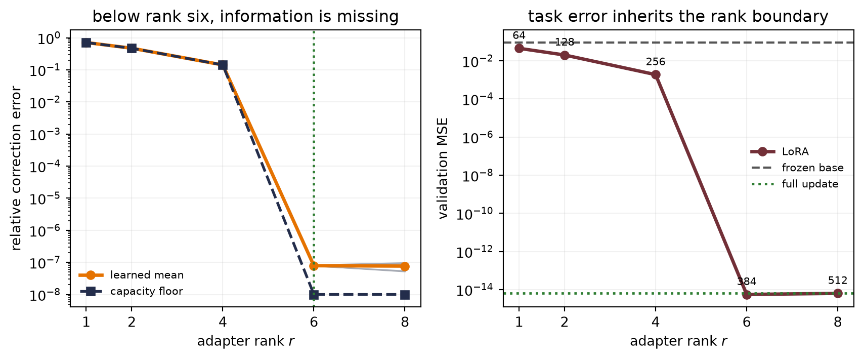

Figure 20.4: LoRA’s rank is a real capacity constraint in a problem constructed to expose it. Five factor initializations converge to the same rank-limited relative update errors (left), closely tracking the analytic best floors from the planted diagonal magnitudes. Validation error (right) falls sharply but remains nonzero below the planted rank six; rank six, rank eight, and the unrestricted full update reach numerical zero. The numbers above the validation points count the trainable adapter values in this small layer.

The failure is orderly. Rank 1 leaves relative correction error \(0.710\); rank 2 leaves \(0.472\); rank 4 leaves \(0.142\). Their mean validation MSEs are \(0.04535,0.02022,\) and \(0.001888\). Rank 6 and rank 8 recover the target to below \(10^{-6}\) relative correction error. The unrestricted update reaches numerical-zero validation MSE and \(2.39\times10^{-7}\) relative correction error. Every frozen base is bitwise intact, and the largest merged–unmerged discrepancy is below \(2\times10^{-6}\).

In this toy \(32\times32\) layer, rank 6 still trains 384 values, 37.5% of a full matrix. The saving is small because the layer is small; real LoRA savings depend on wide matrices, small ranks, and which layers are targeted. The experiment was also built from a low-rank shift. If the chosen rank cannot capture the correction the task needs, some error will remain.

20.4 Quantization: put weights on a smaller grid

PEFT restricts which values may change. Quantization asks how precisely values must be represented. If a tensor contains \(N\) values stored at \(b\) bits each, its ideal packed payload is

\[ \text{payload}=\frac{Nb}{8}\ \text{bytes}. \tag{20.9}\]

One billion FP16 weights therefore require 2 GB in decimal units; an ideal packed 4-bit payload requires 0.5 GB. Those are weight-payload lower bounds, not complete checkpoints or working-memory forecasts. Scales, zero-points, unquantized tensors, packing alignment, activations, and caches remain.

Here a tensor’s dtype becomes more than a software label: fewer nominal bits change both representable values and storage arithmetic. Appendix B covers dtype, shape, stride, and physical layout; Appendix C connects FP16, BF16, rounding, and mixed precision to the finite representations first encountered in Chapter 5.

Start with signed symmetric uniform quantization of a real-valued tensor \(\matr{W}\). For \(b\) bits, let

\[ Q=2^{b-1}-1, \qquad s=\frac{\max_{ij}|W_{ij}|}{Q}. \]

Quantize and reconstruct by

\[ q_{ij}=\operatorname{clip}\!\left( \operatorname{round}(W_{ij}/s),-Q,Q \right), \qquad \hat W_{ij}=s q_{ij}. \tag{20.10}\]

\(s\) is the distance between adjacent real-valued grid points. This symmetric choice uses codes \(-Q,\ldots,Q\): \(2^b-1\) levels, leaving the most-negative two’s-complement code unused so the endpoints remain balanced around zero. With the maximum used for calibration, values are not clipped beyond the selected range; nearest rounding gives \(|W_{ij}-\hat W_{ij}|\le s/2\). One extreme value increases \(s\) for everything sharing that scale, so small values may all round to zero.

If every value is zero, choose any positive sentinel scale, say \(s=1\), and store zero codes. A constant affine range likewise needs a separately defined convention; the range formula below otherwise divides by zero.

An affine grid also stores an integer zero-point \(z\):

\[ q=\operatorname{clip}\!\left( \operatorname{round}(w/s)+z,q_{\min},q_{\max} \right), \qquad \hat w=s(q-z). \tag{20.11}\]

For a nonconstant calibrated interval \([w_{\min},w_{\max}]\), a standard choice is

\[ s=\frac{w_{\max}-w_{\min}}{q_{\max}-q_{\min}}, \qquad z=\operatorname{clip}\!\left( \operatorname{round}\!\left(q_{\min}-\frac{w_{\min}}{s}\right), q_{\min},q_{\max} \right). \]

The zero-point lives in integer-code coordinates. Mixing it with a real-valued offset (subtracting \(z\) before dividing by \(s\), then adding \(z\) after dequantization) is a units error.

One scale can erase a quiet channel

Scale granularity changes the trade: per-tensor quantization shares one scale across an entire matrix. Per-row quantization gives each output row its own scale; for a linear layer this is often called per-output-channel quantization. More scales cost metadata, but a large row no longer sets the grid spacing for a small row.

The next audit creates a \(64\times256\) weight matrix whose row ranges span \(0.01\) to \(10\). It compares 8-bit and 4-bit symmetric grids, either global or per-row, on 4,096 fixed Gaussian inputs. The code reports relative weight error, relative layer-output error, the distribution of row errors, and ideal packed payload plus FP32 scale metadata. It reports no runtime; the simple Python arithmetic is not a quantized production kernel.

1. Fix the audited weight matrix at 64 output rows and 256 input columns.
2. Define the reusable helpers: make_quantization_problem, symmetric_quantize, and run_quantization_audit.
3. Compare per-tensor and per-row symmetric quantization, including output error and metadata.

# [1]
QUANT_D_IN, QUANT_D_OUT = 256, 64


# [2]
def make_quantization_problem(
    seed: int = 1701,
) -> tuple[torch.Tensor, torch.Tensor]:
    generator = torch.Generator().manual_seed(seed)
    directions = torch.randn(QUANT_D_OUT, QUANT_D_IN, generator=generator)
    directions = directions / directions.abs().amax(dim=1, keepdim=True)
    row_ranges = torch.logspace(-2, 1, QUANT_D_OUT).unsqueeze(1)
    weights = directions * row_ranges
    inputs = torch.randn(4096, QUANT_D_IN, generator=generator)
    return weights, inputs


def symmetric_quantize(
    weights: torch.Tensor, bits: int, per_row: bool
) -> tuple[torch.Tensor, torch.Tensor, torch.Tensor]:
    qmax = 2 ** (bits - 1) - 1
    scale = (
        weights.abs().amax(dim=1, keepdim=True) / qmax
        if per_row else weights.abs().amax() / qmax
    )
    scale = torch.where(scale == 0, torch.ones_like(scale), scale)
    codes = torch.clamp(torch.round(weights / scale), -qmax, qmax).to(torch.int8)
    reconstructed = codes.float() * scale
    return codes, reconstructed, scale


@torch.no_grad()
def run_quantization_audit() -> list[dict]:
    weights, inputs = make_quantization_problem()
    reference = inputs @ weights.T
    rows = []
    for bits in (8, 4):
        for per_row in (False, True):
            codes, reconstructed, scale = symmetric_quantize(
                weights, bits, per_row
            )
            row_errors = (
                torch.linalg.norm(reconstructed - weights, dim=1)
                / torch.linalg.norm(weights, dim=1)
            )
            payload_bytes = codes.numel() * bits / 8
            metadata_bytes = scale.numel() * 4
            rows.append({
                "bits": bits,
                "granularity": "per-row" if per_row else "per-tensor",
                "weight_error": (
                    torch.linalg.norm(reconstructed - weights)
                    / torch.linalg.norm(weights)
                ).item(),
                "output_error": (
                    torch.linalg.norm(inputs @ reconstructed.T - reference)
                    / torch.linalg.norm(reference)
                ).item(),
                "row_errors": row_errors.numpy(),
                "row_ranges": weights.abs().amax(dim=1).numpy(),
                "payload_bytes": int(payload_bytes),
                "metadata_bytes": int(metadata_bytes),
                "total_bytes": int(payload_bytes + metadata_bytes),
            })
    return rows


quant_rows = run_quantization_audit()
print("bits  scheme       w err   out err  med row  max row  payload  meta  total")
# [3]
for row in quant_rows:
    print(
        f"{row['bits']:>4}  {row['granularity']:<10}  "
        f"{row['weight_error']:.4f}      {row['output_error']:.4f}      "
        f"{np.median(row['row_errors']):.4f}      {row['row_errors'].max():.4f}  "
        f"{row['payload_bytes']:>7,}  {row['metadata_bytes']:>8,}  "
        f"{row['total_bytes']:>5,}"
    )

bits  scheme       w err   out err  med row  max row  payload  meta  total
   8  per-tensor  0.0213      0.0213      0.2213      1.0000   16,384         4  16,388
   8  per-row     0.0069      0.0069      0.0067      0.0096   16,384       256  16,640
   4  per-tensor  0.2688      0.2695      1.0000      1.0000    8,192         4  8,196
   4  per-row     0.1228      0.1223      0.1225      0.1772    8,192       256  8,448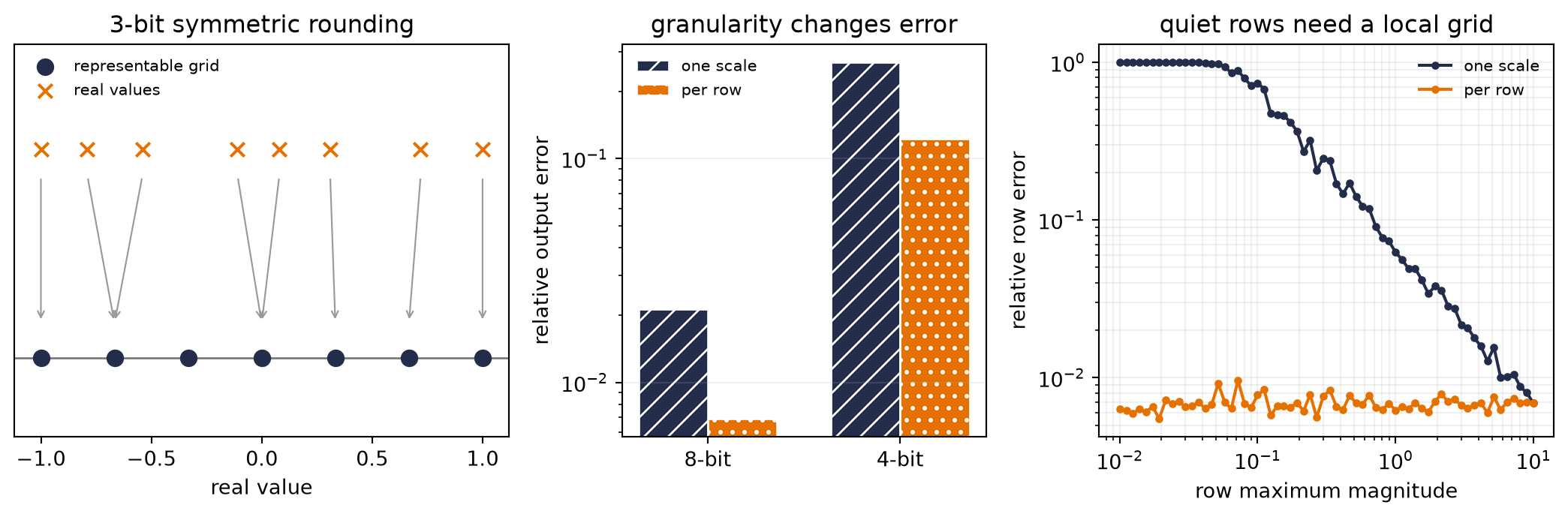

Figure 20.5: Quantization is a grid plus a granularity decision. A 3-bit symmetric example (left) rounds real values to seven levels. In the unequal-row audit, per-row scales reduce relative layer-output error at both bit widths (center). At 8 bits, the global scale entirely erases the smallest rows (relative error 1) while per-row error stays near 0.7% across ranges (right). The improvement costs 256 rather than 4 bytes of FP32 scale metadata.

Watch the mechanism: seven ticks for eight weights

Eight weights, seven ticks: two pairs already share a tick. What pulls them apart, and what does that cost?

These eight weights and this 3-bit grid are the left panel of the figure above — values rounded onto grid = np.arange(-3, 4) / 3. Every other number here is computed from them.

b

2348

b = 3 bits

\( \displaystyle \widehat{w} = \class{qg-s}{s}\,\operatorname{round}(\parameterpart{w}/\class{qg-s}{s}), \qquad \class{qg-s}{s} = \frac{\max|\parameterpart{w}|}{\class{qg-Q}{Q}}, \qquad \class{qg-Q}{Q} = 2^{b-1}-1 \)

Back to three bits: the pairs merge again; payload falls to 0.375 GB.

The calculation is readable without playback. Opening this panel loads the optional controls.

Payload is the chapter's Nb/8 lower bound — bytes of codes, not a checkpoint size and not a speed.

Scope and caveats

One tensor, one scale: s is set by the largest weight and every weight shares it — which is why ±1.00 are the only two the grid leaves alone, and why at seven ticks two pairs cannot be told apart. Opening the grid is this panel's demonstration, not the chapter's remedy: at 8 bits the same rule gives Q = 127, 255 ticks, s = 0.0079 and no error above 0.0039, but the bits are the price the closing beat writes down — 0.375 GB per billion weights at three bits against 1 GB at eight — and the chapter's own next step is per-row scales and zero-points, not more bits. Those and the affine grid are out of scope here; the 64 × 256 audit whose errors the figure's other two panels report is not reproduced, and nothing on this picture measures it. b is the one control: the timeline moves it, 3 → 8 → 3, and dragging it to 2, 3, 4 or 8 pauses playback and recomputes every tick, dot, bar and number from the chapter's rule. The reconstructions (−1, −0.667, −0.667, 0, 0, 0.333, 0.667, 1), the eight errors, the largest of them 0.127 against the bound s/2 = 0.167, the two collisions, the 8-bit grid and the payload are computed here from the cell's own numbers; the chapter prints none of them. The weights are drawn in the colour reserved for a learnable parameter because that is what they are; the grid is a rule, not a thing that learns, and the wine bar is the move the rule makes. Three marks are this panel's own drawing devices and not the chapter's: the dashed ring around a pair that shares a tick; the empty socket that ring becomes when the grid opens, tied by a short dashed line to each of the two dots that left it; and the 8-bit grid drawn as its 255 ticks where the pane can separate them and as a band where it cannot, with the count written once under the picture either way.

Check yourself. Add one outlier weight, 4.0, to this tensor and keep 3 bits. What happens to the original eight weights?

They collapse onto three ticks. The scale becomes s = 4/3 ≈ 1.333, so the eight weights round to −1.333, −1.333, 0, 0, 0, 0, 1.333, 1.333: four of them become exactly zero. One large weight sets the grid for everyone, which is why the chapter turns to per-row scales next.

Transcript and keyboard help

1. Collide. The picture opens on the answer-in-waiting: the 3-bit grid, seven ticks 0.333 apart from −1.00 to 1.00, and the eight weights already standing on their nearest ticks as orange dots. Two ticks carry two dots each, stacked, and a dashed wine ring draws itself around each stack. Those two ticks are named by what the weights became: −0.667 and 0.
2. Where they came from. Four open orange ghosts rise at −0.79, −0.54, −0.11 and 0.08, each with its value written above it, and a wine bar grows from each ghost to the tick it landed on. Four different weights, two numbers.
3. The bound. The four values retire; the other two moved weights, 0.31 and 0.72, take their bars; each tick's basin — everything within s/2 = 0.167 of it — is washed alternately; a bracket measures that half-width from the one tick the dots left free; and 0.127, the longest move on the picture, is written under the bar that is it. s is washed in the formula.
4. Open the grid. The slider rises from 3 to 8 bits and the basins, the bracket and the bars clear. Seven ticks give way to 255 at a spacing of 0.0079, too fine to draw tick by tick at a phone's width, where the grid becomes a band instead; every dot glides to a tick of its own and the two stacks come apart. Each ring stays behind as an empty socket, tied by a dashed line to the two dots that left it, and the four values relight over their own dots. Q is washed in the formula.
5. The price. The slider falls back to 3, the grid returns to seven ticks, the dots glide home and re-stack inside the two rings, and the payload line is written: 0.375 GB per billion weights at three bits, against 1 GB at eight. The grid is yours after that: set b to 2, 3, 4 or 8 and every mark is recomputed.

Silent; paused initially; 1.5× playback. Focus the animation pane: Space or K plays/pauses, arrows seek between beats, Home/End jump, Escape pauses. The scrubber and speed menu also work by keyboard. The b slider is the one parameter control: focus it and its arrow keys move b by one stop, pausing playback and recomputing every mark; they never seek the timeline. A seek or Play hands b back to the timeline. Reduced-motion mode holds each beat’s state: every dot stands on its beat’s tick, never between.

The global 8-bit grid has only \(2.13\%\) relative output error overall, which sounds reassuring until we inspect rows: the median relative row error is \(22.13\%\), and the quietest rows are reconstructed as all zeros. Per-row scales lower overall output error to \(0.689\%\) and maximum row error below \(0.964\%\). At 4 bits, per-row scales improve output error from \(26.95\%\) to \(12.23\%\), but do not make the approximation exact.

The packed 4-bit codes require 8,192 bytes. One FP32 scale brings the global total to 8,196 bytes; 64 row scales bring it to 8,448. The live torch.int8 tensor in this teaching cell occupies one byte per code; it is not physically packed into nibbles. Equation 20.9 is the payload a packing format could achieve.

WarningA smaller checkpoint is not automatically faster

Bit count does not determine latency by itself. Real speed depends on supported kernels, hardware, packing, dequantization, memory bandwidth, batch shape, and which tensors remain in higher precision. Dettmers and colleagues even reported cases where LLM.int8() overhead made smaller models slower than FP16. Measure the target system; do not turn a file-size ratio into a runtime claim. Appendix C draws that distinction with the Roofline model and matched evidence.

Watch the mechanism: one scale can erase a quiet row

Can an 8-bit grid erase every weight in a row without clipping any weight?

Keep the audit's bit width fixed. Follow its quietest row's range while the loudest row sets a shared scale, then give the quiet row its own scale.

\( s_{\mathrm{tensor}}=\dfrac{\max_{ij}|\parameterpart{W_{ij}}|}{Q} \) \( s_i=\dfrac{\max_j|\parameterpart{W_{ij}}|}{Q} \) \( |\residualpart{w-\widehat w}|\leq\dfrac{s_i}{2} \)

Per-row scaling protects this quiet range. It does not guarantee exact weights, accuracy, or faster inference.

The range argument is readable without playback. Opening this panel loads the optional controls.

This is the audit's declared range argument, not a plot of sampled weights or a new error measurement.

Scope and caveats

The ruler keeps a fixed quiet-row zoom. Local ticks show every 32nd code plus endpoints, not every grid level. The traced positive endpoint denotes maximum magnitude, not an assumed signed sample. A local scale does not reconstruct every weight exactly; the rounding bound assumes no clipping. FP32 scale metadata grows while the 8-bit code payload stays fixed. Storage savings do not establish runtime speed.

Check yourself. Suppose the loud row's largest weight were 1 instead of 10. Under one shared 8-bit scale, how many distinct codes could the quiet row use?

Three: −1, 0 and 1. The shared spacing would be 1/127 ≈ 0.00787, so the quiet row's largest weight, 0.01, is only 1.27 spacings from zero. Better than one code — and still nowhere near the 255 a per-row scale gives it.

Transcript and keyboard help

1. Predict whether a shared 8-bit grid can erase the quiet row without clipping. The audit has 64 rows of 256 weights.
2. The loudest row reaches magnitude 10. With Q equal to 127, its shared scale is 10 divided by 127, approximately 0.07874.
3. The quiet row lies between minus 0.01 and plus 0.01. Its entire range is strictly inside the zero bin, whose half-width is approximately 0.03937.
4. The interval contracts to zero: every quiet weight receives integer code zero, even though the row is within the calibrated range.
5. Keep eight bits but use the quiet row's own maximum. Its scale is 0.01 divided by 127. The zero bin becomes one thousand times narrower on the same ruler.
6. The maximum-magnitude endpoint maps to code 127 and back to 0.01. This endpoint is exact, but other weights generally still round; their error is at most half the local spacing, approximately 0.00003937.
7. One FP32 scale costs 4 bytes. Sixty-four row scales cost 256 bytes. The 16,384-byte 8-bit code payload is unchanged.
8. The mechanism explains the quiet-row failure and repair. It does not replace the audit's measured output errors or promise faster inference.

Silent; paused initially; 1.5× playback. Focus the animation pane: Space or K plays/pauses, arrows seek between beats, Home/End jump, Escape pauses. The scrubber and speed menu also work by keyboard. Reduced-motion mode holds each beat's state instead of moving between them.

What a quantization workflow protects

Post-training quantization (PTQ) chooses a representation after the base model has trained. It may use calibration inputs, but it does not run ordinary end-to-end training again. Our uniform audit used only weight ranges. More sophisticated PTQ methods protect behavior measured on calibration data. For example, a method can choose the quantized weights that best preserve a layer’s outputs on calibration inputs. For a layer \(\matr{W}\in\mathbb{R}^{d_{\mathrm{out}}\times d_{\mathrm{in}}}\) and \(n\) calibration activations \(\matr{X}\in\mathbb{R}^{d_{\mathrm{in}}\times n}\), these weights solve the layerwise weight-only problem

\[ \hat{\matr{W}} =\argmin_{\widetilde{\matr{W}}\in\mathcal{Q}} \left\|\matr{W}\matr{X} -\widetilde{\matr{W}}\matr{X}\right\|_F^2, \tag{20.12}\]

where \(\widetilde{\matr{W}}\) has the same shape as \(\matr{W}\) and \(\mathcal{Q}\) is the chosen quantized set. The objective protects layer outputs, not ordinary weight MSE and not the original task loss. GPTQ is one method that solves this problem approximately. AWQ uses activation evidence to choose channel scaling that protects salient weights. These methods make the calibration distribution part of the result.

Quantization-aware training (QAT) instead inserts fake quantize–dequantize operations into the forward pass while retaining higher-precision shadow weights for optimization. Because rounding is nondifferentiable, training uses a surrogate gradient such as a straight-through estimator. QAT is not integer-only training; conversion to integer execution remains a separate, kernel-dependent step.

Weight-only and weight–activation quantization also address different bottlenecks. A weight-only method leaves activations and the autoregressive key/value cache at their chosen compute precision. LLM.int8(), by contrast, quantizes both matrix inputs and weights while routing a small activation-outlier subspace through FP16 in its studied regime. “8-bit method” is not a complete algorithm description.

QLoRA: compose a frozen grid with a trainable delta

QLoRA places the two major levers side by side. Store a pretrained base in blockwise 4-bit NormalFloat (NF4), dequantize blocks to BF16 for matrix multiplication, and train higher-precision LoRA factors:

\[ \vect{h} =\operatorname{Dequant}_{\mathrm{NF4}}(\matr{W}_q)\vect{x} +\frac{\alpha}{r}\matr{B}(\matr{A}\vect{x}). \tag{20.13}\]

The base codes \(\matr{W}_q\) remain frozen. The gradient passes through the dequantized computation to the LoRA path, but ordinary updates do not rewrite the 4-bit base. QLoRA is therefore not QAT of the backbone, and “4-bit storage” does not mean every multiply or accumulator is 4-bit.

NF4 uses a nonuniform codebook with denser resolution where a standardized normal distribution places more probability mass, plus an exact zero. Its information-theoretic argument applies to block-normalized, approximately zero-centered normal weights; it is not a universal optimal grid for arbitrary tensors.

Figure 20.6: QLoRA composes quantized storage with low-rank training without conflating the two. A frozen blockwise NF4 base is dequantized to the compute dtype for the main matrix multiplication. Higher-precision A and B factors form a trainable low-rank branch, and only that branch has optimizer state. The sum defines the adapted layer; storage dtype, compute dtype, and trainable dtype are separate choices.

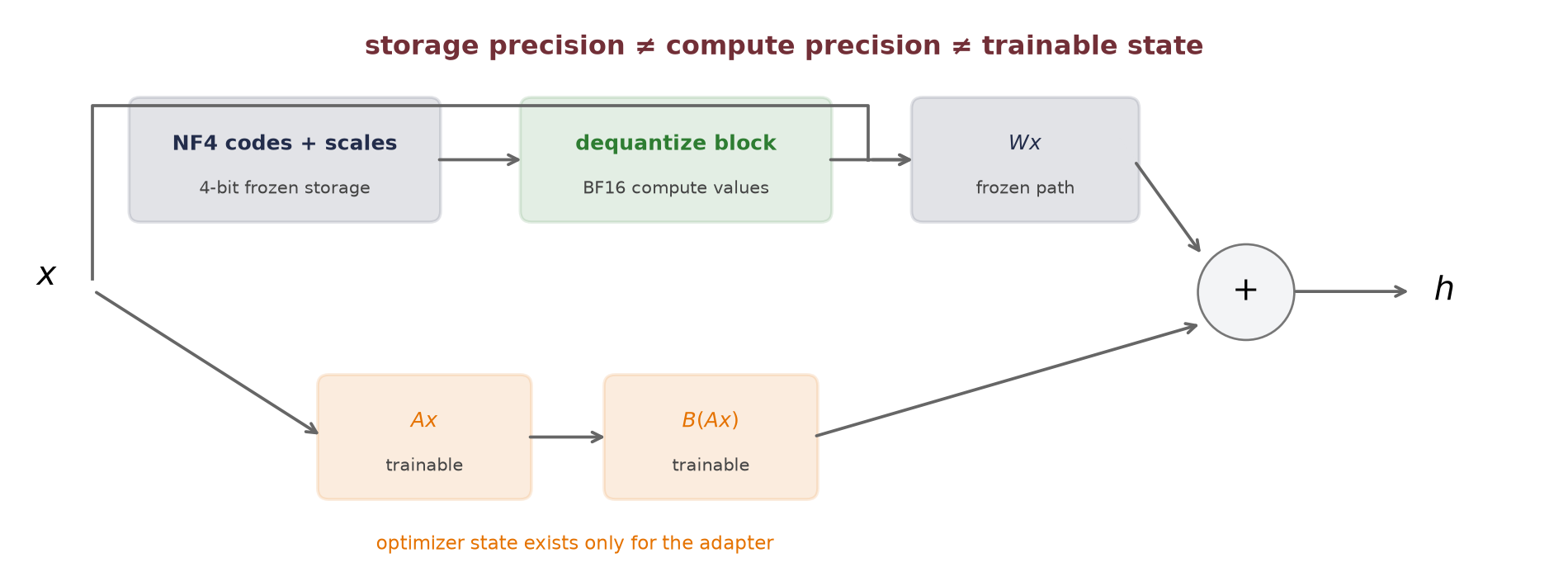
QLoRA also uses double quantization: it quantizes its quantization constants. With the paper’s illustrative group sizes, FP32 constants for each 64-weight block cost \(32/64=0.5\) bits per weight. Storing those constants at 8 bits and adding one FP32 second-level constant per 256 first-level constants costs

\[ \frac{8}{64}+\frac{32}{64\cdot256}=0.126953 \quad\text{bits per weight}, \]

a saving of \(0.373047\) bits per weight. That number belongs to those block sizes; it is not a universal number of gigabytes. Paged optimizers address transient memory spikes in the paper’s implementation, while the LoRA factors still carry their own gradients and optimizer state.

NoteQLoRA is a composition, not a new objective

NF4 decides how the frozen foundation is stored; LoRA decides where task gradients may write. The supervised, preference, or other loss still decides what behavior is rewarded. A parameter-efficient route can optimize a poor objective just as efficiently as a good one.

20.5 Choose by the cost you need to reduce

Method	Task state and permitted writes	Main consequence
Hard prompt / ICL	State in ordinary context; no gradients during use	No learned task checkpoint; longer context
RAG	State in index and retrieved context; writes depend on design	Fresher evidence; retrieval failure surface
Prompt tuning	State in continuous input vectors; write prompt vectors, plus any unfrozen head	Small learned state; virtual positions remain
Prefix / adapters	State in per-layer prefixes or bottlenecks; write added modules	Small checkpoint; extra inference path
LoRA	State in \(\matr{A},\matr{B}\); write factors, plus any unfrozen head	Conditionally mergeable; rank bottleneck
Full fine-tuning	State in a changed backbone; write all permitted parameters	Maximum update freedom; one full task copy
PTQ	No task state: representation only; no gradients in ordinary PTQ	Smaller weight representation; approximation error
QLoRA	Task state in LoRA factors; codes/scales describe the frozen base; write factors plus any unfrozen head	Smaller base representation during PEFT; mixed dtypes

A practical instinct remains useful: when a carefully evaluated prompt or retrieval pipeline solves the task, avoid fine-tuning merely because it is available. Treat that as a search heuristic, not a law. A stable format change may fit a small adapter; genuinely new knowledge may belong in retrieval or further training; a severe source-coverage mismatch may defeat all of them.

PEFT changes the cost after we choose transfer; it does not settle whether transfer helps. As in Chapter 10, that question needs an explicit comparison on the target task. A frozen foundation cannot guarantee a reliable representation of what its source data never covered, and a low-rank update does not guarantee that scarce target labels can build the missing feature. Quantization preserves or damages an existing computation; it does not add coverage.

WarningTrainable parameters are not total memory

During PEFT, the frozen base still occupies memory and backpropagation still stores or recomputes activations through it. During generation, context and key/value caches can dominate memory in different regimes. Optimizer dtype and implementation change the total. Report trainable state, base storage, transient training memory, context length, and measured runtime separately. One percentage cannot stand in for all five.

Parameter efficiency also does not guarantee immunity to forgetting or harmful behavior. Restricting an update constrains which coordinates or directions are available; it does not bound the update’s magnitude or certify what the movement preserves. Evaluation must include the target task, retained capabilities that matter, calibration or distribution shifts, and the actual deployment representation.

20.6 What should the update optimize?

Where the update lives is not what the update optimizes. Prompt vectors, low-rank matrices, and full fine-tuning decide where task gradients may write. Quantization decides how values are stored. None decides which answer is helpful, harmless, honest, or preferred.

Chapter 21 will keep the adaptation machinery and change the question from which parameters move? to which objective should move them? Instruction tuning, preference learning, and alignment methods are claims about supervision and objectives, not automatic consequences of choosing LoRA or a full checkpoint.

NoteCheck yourself

Close the book for one minute and separate adaptation’s three costs.

• Where can task-specific state live when the backbone is frozen?
• What does LoRA’s rank constrain, and what does quantization change instead?
• Why can a method reduce stored bits without reducing every inference cost?

20.7 Okay, so: adaptation has three separate costs

1. Adaptation has three costs. Backbone storage, incremental task state, and transient work must be reported separately. Zero trainable weights and fewer stored bits do not mean zero inference or training cost.
2. Prompting changes context, not weights. The five-seed permutation study closely tracks the analytical information ceilings while the weights stay bitwise fixed during evaluation. RAG is another context lever, with a separate retrieval failure surface.
3. PEFT restricts where gradient updates may write. Prompt tuning, prefixes, adapters, BitFit, and LoRA impose different parameterizations; they are not interchangeable labels for “small fine-tuning.”
4. LoRA learns a low-rank correction. Its trainable count is \(r(d_{\mathrm{in}}+d_{\mathrm{out}})\) per targeted matrix, and its rank is a real capacity limit. The planted rank-six experiment fails exactly where it should.
5. Quantization is a grid, a granularity, and a workflow. Per-row scales rescue quiet rows in the controlled audit, but consume metadata. Payload size does not predict runtime without kernels and hardware.
6. QLoRA composes representation and adaptation. A frozen NF4 base is dequantized for compute while higher-precision LoRA factors train. Storage dtype, compute dtype, and trainable dtype are distinct.
7. The choice still needs evaluation on the target task. None of these methods creates source knowledge for free.

Sources and further reading

• Brown et al., Language Models are Few-Shot Learners: GPT-3’s zero-, one-, and few-shot evaluation and its model-scale dependence.
• Min et al., Rethinking the Role of Demonstrations: What Makes In-Context Learning Work?: controlled ablations of demonstration inputs, labels, and formatting that qualify simple imitation accounts.
• Lewis et al., Retrieval-Augmented Generation for Knowledge-Intensive NLP Tasks: learned retrieval combined with a pretrained generator.
• Houlsby et al., Parameter-Efficient Transfer Learning for NLP: bottleneck adapters inserted into a frozen Transformer.
• Li and Liang, Prefix-Tuning: Optimizing Continuous Prompts for Generation: trainable per-layer prefixes for generation.
• Lester et al., The Power of Scale for Parameter-Efficient Prompt Tuning: input-level soft prompts and the scoped T5 scale study.
• Ben-Zaken et al., BitFit: Simple Parameter-Efficient Fine-Tuning for Transformer-Based Masked Language-Models: bias-term updates plus the task-specific classifier in the original experiments.
• Hu et al., LoRA: Low-Rank Adaptation of Large Language Models: the low-rank update parameterization, initialization, and merge.
• Wei et al., Chain-of-Thought Prompting Elicits Reasoning in Large Language Models: scoped gains from prompting with intermediate reasoning steps.
• Turpin et al., Language Models Don’t Always Say What They Think: Unfaithful Explanations in Chain-of-Thought Prompting: controlled evidence that visible explanations can omit causal influences on predictions.
• Greshake et al., Not What You’ve Signed Up For: Compromising Real-World LLM-Integrated Applications with Indirect Prompt Injection: the attack surface created when untrusted retrieved data can act as instructions.
• Jacob et al., Quantization and Training of Neural Networks for Efficient Integer-Arithmetic-Only Inference: affine quantization and the fake-quantization training pattern.
• Dettmers et al., LLM.int8(): 8-bit Matrix Multiplication for Transformers at Scale: mixed-precision decomposition for activation outliers, and measured overhead caveats.
• Frantar et al., GPTQ: Accurate Post-Training Quantization for Generative Pre-trained Transformers: calibration-output-aware, layerwise weight-only PTQ.
• Lin et al., AWQ: Activation-aware Weight Quantization for LLM Compression and Acceleration: activation evidence for protecting salient weights.
• Dettmers et al., QLoRA: Efficient Finetuning of Quantized LLMs: NF4, double quantization, paged optimizers, and LoRA over a frozen quantized base.

Exercises

1. (Pencil.) A model has 24 matrices of shape \(4096\times4096\). LoRA targets each with rank 16. Compute full and adapter value counts, the adapter fraction, and FP16 adapter bytes. Then compute the ideal 4-bit base payload. Add one FP32 scale per block of 64 weights and explain which deployment costs the count still leaves out.
2. (Code.) Reproduce the frozen-context experiment, then randomize demonstration order, repeat one group with the same label, and finally insert a contradictory label for a repeated group. Predeclare which interventions preserve Equation 20.2 and which make it inapplicable. Report all seeds and verify bitwise parameter identity before interpreting a difference.
3. (Pencil.) (a) Prove \(\operatorname{rank}(\matr{B}\matr{A})\le r\). (Code.) (b) Extend the rank-capacity audit with a planted rank-10 correction and ranks \(2,6,10,14\). Audit gradients after the first backward pass for random \(\matr{A}\) with zero \(\matr{B}\), and for both factors zero. Verify merged–unmerged equality.
4. (Pencil.) (a) Quantize \([-1.2,-0.3,0.0,0.5,1.7]\) onto a signed 4-bit symmetric grid, showing \(Q,s,q,\) and \(\hat w\). Then construct an affine 8-bit grid for a nonnegative interval. (Code.) (b) On the chapter’s unequal-row matrix, compare calibration and held-out output error after inserting one new outlier row.
5. (Audit.) For each of three cases (fresh facts with citations, a stable output format, and a target domain absent from the source data) choose a first experiment among prompting/RAG, PEFT, full tuning, and quantization. State where task state lives, which cost it reduces, what it cannot repair, and one retained behavior you would evaluate. Finally explain why none of those choices answers the Chapter 21 question of which behavior deserves reward.