18  The BERT Moment: Pretraining as the New Regime

Chapter tools Lecture 10.1 · Vision Transformer·Lecture 10.2 · Pretrained Transformer Models·Lecture 10.3 · Scaling Decoder Transformer Models·Download notebook·Open in Colab (opens in a new tab)

In Chapter 10, we compared training from scratch with adapting features learned on another task. For language, task-specific labels can be scarce while unlabeled text is available. Can that text provide a useful training signal before we introduce a downstream task?

Masked language modeling constructs such a signal from the sequence itself. Replace bank in “the boat reached the bank” or “the bank approved the loan” and predict the original token from the corrupted input. Both examples have the same target word, but different contexts. The task provides token targets without requiring separate labels for word senses.

That move depends on what Chapter 16 showed: visibility is a modeling decision. A next-token model used a causal triangle because looking right would reveal its target. A representation model can instead let every nonpadding token consult both sides, provided enough selected positions are masked or replaced in the input that copying cannot solve the whole task. Full visibility over a corrupted input, scored on the original selected tokens, gives masked language modeling (MLM), and pretraining on raw text changed the default workflow from “initialize and train” to “pretrain, then adapt.”

18.1 Separate controls, not one mask

Bidirectional Encoder Representations from Transformers (BERT) uses a few special tokens. [CLS] is a learned summary placeholder, [SEP] marks a boundary, and [PAD] fills unused batch slots. Consider six positions:

\[ [\text{CLS}],\quad \text{the},\quad \text{bank},\quad \text{rose},\quad [\text{SEP}],\quad [\text{PAD}]. \]

There are four distinct decisions in play.

1. Attention visibility decides which key positions each query may use. A causal decoder blocks future keys; a BERT encoder permits all nonpadding keys.
2. The MLM target selector chooses which ordinary positions contribute loss.
3. The corruption branch replaces some selected tokens by [MASK], replaces some by random tokens, and deliberately leaves some unchanged.
4. The padding mask prevents real tokens from routing information from placeholder slots used only to make batch shapes rectangular.

1. Construct causal and full visibility beside a separate MLM selector.

# [1]
import copy
import itertools

import matplotlib.pyplot as plt
import numpy as np
import torch
from torch import nn
import torch.nn.functional as F
torch.set_num_threads(4)  # pinned: results depend on the CPU thread count

tokens = ["[CLS]", "the", "bank", "rose", "[SEP]", "[PAD]"]
nonpadding = np.array([1, 1, 1, 1, 1, 0], dtype=bool)
causal = np.tril(np.ones((6, 6), dtype=int)) * nonpadding[None, :]
full = np.ones((6, 6), dtype=int) * nonpadding[None, :]
selector = np.zeros((1, 6), dtype=int)
selector[0, 2] = 1

Figure 18.1: Visibility and supervision are separate controls. A causal decoder sees a lower triangle (left); BERT-style attention sees every nonpadding key (center). The MLM selector marks one selected target position (right).

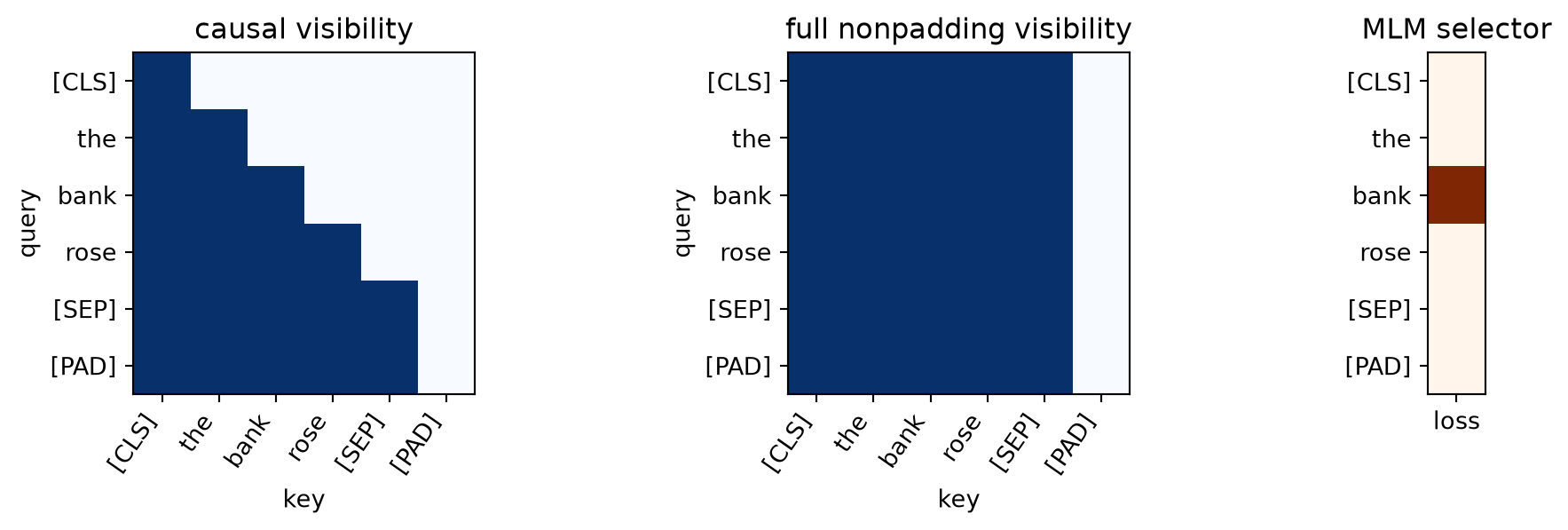
The center matrix contains no future-blocking triangle. Every nonpadding query can route from every nonpadding key, including itself. That is what bidirectional means here: a token’s representation can jointly use left and right context in every layer. It does not mean running two separate recurrent networks, and it does not define a left-to-right probability for the whole sentence.

Only padding keys are blocked in the drawing. A [PAD] query row can still produce an output, which downstream computation ignores; real queries, however, can never retrieve padding as information.

Now suppose bank is selected and replaced:

\[ [\text{CLS}]\ \text{the}\ [\text{MASK}]\ \text{rose}\ [\text{SEP}]\ [\text{PAD}]. \]

Every ordinary token may attend to [MASK], because [MASK] is an input token, not an attention prohibition. Only the selector says that position 2 contributes MLM loss. The padding mask separately blocks the final slot as a key. Reusing mask for visibility, selection, corruption, and padding is convenient shorthand, and a reliable source of bugs.

WarningThe copy trap

If full attention received the original token at every selected position, the model could copy answers through the residual stream. BERT’s policy corrupts 90% of selected sites, so copying cannot solve the whole task; the deliberate 10% unchanged branch has a separate purpose below. Conversely, replacing a token by [MASK] does not make it invisible; its neighbors still see the placeholder and one another. Always audit visibility, selection, corruption, and padding separately.

18.2 Text supplies supervision

In ordinary supervised learning, an external label \(y\) accompanies input \(x\). Masked language modeling derives both from one unlabeled sequence: the corrupted sequence is the input, and the original selected tokens are the targets. This is self-supervised learning: the supervision is constructed from the data rather than supplied by a human annotator.

NoteSelf-supervised does not mean target-free

The method still has labels and a loss. What changes is their origin. The clean text supplies a target for every selected position, so a large corpus can create many training examples without a task-specific annotation campaign.

This idea was part of a broader 2018 convergence, not a solitary invention. Table 18.1 sets four of its works side by side.

Table 18.1: Four 2018 works, with the pretraining signal of each and what moved downstream.

Work	Pretraining signal	What moved downstream
ELMo	Forward and backward LSTM language models	Fixed contextual features
ULMFiT	Causal language modeling	The entire adapted language model
GPT	Causal Transformer language modeling	A pretrained Transformer plus task head
BERT	Masked tokens in full context, plus NSP	A deeply bidirectional Transformer encoder plus task head

ELMo demonstrated that a word’s useful vector should depend on its sentence. ULMFiT supplied a robust recipe for adapting a pretrained language model rather than freezing it. GPT paired Transformer pretraining with supervised fine-tuning. BERT’s decisive change was to pretrain every encoder layer with joint left-and-right context. The workflow mattered as much as the architecture: learn broadly from raw text first, then spend scarce labels on adaptation.

18.3 The masked-language-model objective

Let a tokenized sequence be

\[ x=(x_1,\ldots,x_T),\qquad x_t\in\{1,\ldots,|V|\}, \]

where \(T\) is sequence length and \(V\) is the vocabulary. Choose a random set \(M\) of eligible positions, then apply a corruption operator \(c\) to obtain \(\widetilde{x}=c(x,M)\). A bidirectional encoder with parameters \(\theta\) produces

\[ H=f_\theta(\widetilde{x})\in\mathbb{R}^{T\times d}. \]

An output head maps each selected hidden state to vocabulary logits. The MLM loss is

\[ \mathcal{L}_{\mathrm{MLM}}(\theta) =- \frac{1}{|M|} \sum_{i\in M} \log p_\theta\!\left(x_i\mid \widetilde{x}\right). \]

Every term conditions on the same jointly corrupted sequence \(\widetilde{x}\), not on its own clean sequence with only \(x_i\) removed. With batches, token IDs have shape \((B,T)\), hidden states \((B,T,d)\), and dense vocabulary logits \((B,T,|V|)\). Boolean selection gathers \(|M|\) rows, so cross-entropy receives selected logits \((|M|,|V|)\) and targets \((|M|,)\). Unselected positions can affect the representations but contribute no direct MLM loss.

Fifteen percent, then 80/10/10

Original BERT selects 15% of eligible tokens. Conditional on selection:

• 80% are replaced by [MASK];
• 10% are replaced by a random vocabulary token;
• 10% remain unchanged.

For 1,000 eligible positions, the expected flow is therefore

\[ 1000\longrightarrow150\longrightarrow \begin{cases} 120 & [\text{MASK}],\\ 15 & \text{random token},\\ 15 & \text{unchanged}. \end{cases} \]

All 150 selected positions are scored against their original token. The 120 mask replacements are 12% of all eligible positions, not the complete supervision rate. Random ordinary-looking replacements force the encoder to cross-check a token against its context rather than trusting the visible identity. The unchanged branch prevents the opposite shortcut: the assumption that every selected ordinary-looking token must be wrong. It also reduces the mismatch between pretraining, where [MASK] exists, and downstream inputs, where it ordinarily does not. An unchanged selected token exposes its answer on purpose; only about 1.5% of all eligible positions follow that branch, and the encoder is not told which normal-looking tokens were selected.

1. Compute the expected two-stage policy counts.
2. Build and audit the five Boolean rows on one illustrative sequence.
3. Report the policy totals.

# [1]
eligible_count = 1_000
selected_count = round(0.15 * eligible_count)
branch_counts = np.array([120, 15, 15])

# [2]
ledger_tokens = [
    "[CLS]", "the", "quiet", "bank", "rose", "after",
    "the", "rain", "today", "[SEP]", "[PAD]", "[PAD]",
]
eligible = np.array([False] + [True] * 8 + [False] * 3)
selected = np.array(
    [False, False, True, False, True, False, False, True, True, False, False, False]
)
mask_sites = np.array(
    [False, False, True, False, False, False, False, True, False, False, False, False]
)
random_sites = np.array(
    [False, False, False, False, True, False, False, False, False, False, False, False]
)
unchanged_sites = selected & ~mask_sites & ~random_sites
assert np.all(selected <= eligible)
assert np.array_equal(selected, mask_sites | random_sites | unchanged_sites)
assert not np.any(mask_sites & random_sites)

# [3]
print(f"direct loss targets: {branch_counts.sum()}")
print(f"[MASK] share of all eligible positions: {branch_counts[0] / 1000:.1%}")

direct loss targets: 150
[MASK] share of all eligible positions: 12.0%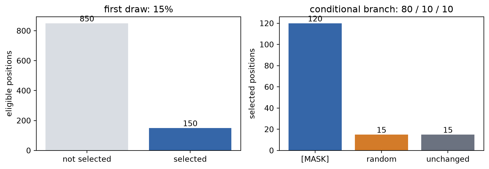

Figure 18.2: Five Boolean rows keep BERT’s controls separate. Eligibility excludes special and padding tokens; selection identifies direct loss targets; three disjoint corruption rows partition the selected sites into mask, random, and unchanged branches. Attention visibility remains full over nonpadding keys and is not encoded by any of these rows. The example deliberately gives each branch only a few positions; the 15% and 80/10/10 rates hold on average over many positions and cannot be read from these twelve.

Watch the mechanism: what is seen, what is scored?

An ordinary-looking token was selected. Does it still contribute to the loss?

Change what the model reads. Keep a copy of what it should predict.

SelectMaskReplaceKeepCompare

Each column: the original above the input BERT reads; ↓ marks a changed position, = an unchanged one. Positions are zero-based.

0[CLS]=[CLS] 1the=the 2quiet↓[MASK]chosen 3bank=bank 4rose↓bankchosen* 5after=after 6the=the 7rain↓[MASK]chosen 8today=todaychosen 9[SEP]=[SEP] 10[PAD]=[PAD] 11[PAD]=[PAD]

* At position 4 the input “bank” is one illustrative random replacement for the original rose.

BERT reads the input copies: all 10 nonpadding tokens can supply context. PAD is blocked as a key. “Chosen” is our bookkeeping, not an extra model input.

Unchanged, but chosenPosition 8: today

In BERT’s inputtodayOne position in the full corrupted context

Saved originaltodayA loss target, not an extra BERT input

Encoder + vocabulary headPrediction at 8Uses every visible context position

Does this position count?Yes: −log p₈(today)Score the original, not the replacement

Today looks ordinary because it was left unchanged, but selected = 1. Its prediction is still scored against the original token today.

The ledger and routes are readable without playback. Opening this panel loads the optional controls.

Inspect the five Boolean ledgers

Position 8: selected; unchanged.

eligible

1

selected

1

mask_sites

0

random_sites

0

unchanged_sites

1

These flags track the outlined position. The last three partition the selected sites; none is an attention-visibility mask.

The four selected positions illustrate branches, not the population’s 15% or 80/10/10 proportions. No model probabilities or measured losses are supplied.

Check yourself. BERT reads “bank” at position 3 and “bank” again at position 4. Which of the two contributes a loss term, and what is its target?

Only position 4: it was selected, so its prediction is scored against the saved original, “rose”. Position 3 was never selected and contributes nothing. The input alone cannot tell you; the selection ledger decides.

Transcript and keyboard help

1. The original sequence is [CLS], the, quiet, bank, rose, after, the, rain, today, [SEP], [PAD], [PAD]. Positions are zero-based. Positions 1–8 are eligible; positions 2, 4, 7, 8 are selected. Each column keeps an original above its input copy; “chosen” marks are reader/training bookkeeping, not an extra encoder input.
2. Apply corruption jointly: replace quiet and rain at positions 2 and 7 with [MASK]; at position 4, use bank as an illustrative random replacement for rose; keep selected today at position 8 unchanged.
3. For masked quiet, the encoder reads [MASK], but its position-2 prediction is scored against original quiet. Selected rain at position 7 follows the same route. For replaced rose, it reads bank, but its prediction is scored against original rose. For unchanged selected today, it reads today and is still scored against today.
4. Unselected bank at position 3 remains visible context but contributes no direct MLM loss. [CLS] and [SEP] also remain visible but are ineligible. [PAD] is ineligible and blocked as an attention key.
5. The encoder reads one jointly corrupted sequence. Every selected position contributes one negative log-probability term; the chapter’s loss averages these terms. Original target labels feed the loss, not an extra input to the encoder. The unchanged branch deliberately leaves its answer visible.

Silent; paused initially; 1.5× playback. Focus the animation pane: Space or K plays/pauses, arrows seek, Home/End jump, Escape pauses. The scrubber and speed menu also work by keyboard. Rays reveal the input, saved-label, and prediction paths in order; this is an explanation of one jointly corrupted input, not separate model runs. Reduced-motion mode uses discrete reveals without moving dots.

Original BERT pre-generated several masked versions of its training examples; RoBERTa later redrew masks as examples were presented. Our controlled lab uses the latter dynamic corruption choice: the same sentence can ask different questions on later passes. Reproducibility therefore requires a separate random generator. Seeding model initialization while leaving the corruption stream implicit is not an exact experiment.

TipAudit the selector before the loss

Print the number of eligible and selected positions, verify that special and padding tokens are excluded, and inspect the realized 80/10/10 proportions over many batches. Then assert that the selected logit and target shapes agree. A loss can decrease while a selector silently trains on padding or on the wrong tokens.

18.4 From a Transformer encoder to BERT

The original BERT input at position \(i\) adds three learned vectors:

\[ z_i=e_{\text{token}(i)}+e_{\text{position}(i)}+e_{\text{segment}(i)}. \]

The token comes from a WordPiece vocabulary: frequent character sequences are stored whole, while rarer words can be assembled from reusable subword pieces.

TipPractice bridge (optional): make the vocabulary learnable

Chapter 12 fixed its vocabulary at individual characters. A full-word vocabulary shortens sequences but gives every rare spelling its own entry. Subword tokenization sits between the two. Byte Pair Encoding (BPE) begins with small symbols, counts adjacent pairs in the training corpus, merges the most frequent pair, and repeats until it reaches a chosen vocabulary budget.

This original toy implementation starts from characters plus an end-of-word marker. Corpus frequencies weight the pair counts; lexicographic order breaks exact ties so the result is reproducible.

Watch the mechanism: every round counts the pairs again

Byte pair encoding merges the most frequent adjacent pair, then repeats. At its first count, w+e has 8, across newest and lower, and l+o has 7, across low and lower. Its first three merges each use 9 weighted occurrences. Which pair is merged fourth?

The loop below starts every round with counts: Counter[tuple[str, str]] = Counter(), a fresh count of the current pieces. Here are its four counted words as tiles.

\( \text{count}(a{+}b)=\sum_{\text{words}}\text{frequency}\times\#\bigl(a\ b\ \text{adjacent}\bigr),\quad \class{pr-recount}{\text{taken on the current pieces every round}} \)

Counts are redone each round: e+s took newest's e, so w+e fell to 2 and l+o won.

The final pieces are readable without playback. Opening this panel loads the optional controls.

Byte pair encoding on the chapter's four-word toy corpus, recounted after every merge; not BERT's WordPiece, which scores merges differently, and no real tokenizer is trained.

Scope and caveats

Every count is computed from the corpus line by the loop below. The chapter's text names only the nine and the seven; the 8, 6 and 2 of w+e are this panel's recount of the same loop. The loop counts fourteen distinct adjacent pairs in round 1. The picture draws two of them and the maximum, and it folds the counts of rounds 3 and 5 into their merges.

The lesson does not rest on the tie-break. With the reverse tie order, w+e keeps 8 through the three nines and drops to 2 after the third merge, and the final pieces are the same. The merge names do change (t+</w>, s+t</w>, e+st</w>, o+w, l+ow): the fourth merge is then o+w, the other 7, not l+o, and w+e still never merges. </w> sorts before letters in lexicographic order. It decides no tie here: every tie in these five rounds is settled by the first piece. With lower counted 3, w+e would tie the three nines and lose to e+s in lexicographic order. The check below takes 4.

An arc marks one adjacent occurrence of a drawn pair, and a bar adds up those occurrences, each weighted by its word's frequency. The dashed outline keeps w+e's first count for comparison; the loop keeps no such record. Where lower's w+e stood, the pair after merge 5 is low+e, counted 2. The loop stops after five merges, a chosen budget, not at any convergence, so no count follows the last merge; the live w+e bar is retired once its last arc is gone.

The panel previews the corpus and the merges that the next cell declares and prints. The printed output remains the authority. BERT's own tokenizer scores merges differently, and practical byte-level tokenizers begin from bytes. A finished merge list is applied in its own order when new text is split. The recount shown here is how that order is found.

Tiles and frequencies are blue, as tokens are in this chapter's other panel. The count the loop makes for w+e is neutral ink, like the level and the stub; the rival l+o is slate and thinner, and every tally also carries its label.

Check yourself. Suppose lower were counted 4 times instead of 2, all else unchanged. Which pair merges first, and what does e+s count in the round after?

w+e: 6 + 4 = 10 beats every 9, and five pairs now tie at 9, since l+o and o+w rise to 5 + 4. The merge fuses w and e in newest and lower, so the next round counts e+s at only the 3 from widest. A merge removes another pair only where the two share a symbol occurrence.

Transcript and keyboard help

1. Four words from the corpus line, in character tiles, each ending in the end-of-word marker </w>: low ×5, lower ×2, newest ×6, widest ×3. At the first count w+e has 8, 6 from newest and 2 from lower, and l+o has 7, 5 from low and 2 from lower. The most frequent adjacent pairs tie at 9: e+s, s+t and t+</w>. Predict which pair is merged fourth.
2. Merge 1 fuses e and s into es, in newest and widest at once. newest's e now sits inside es, so the arc over its w and e snaps, leaving a dashed stub. The loop then counts again on the current pieces: w+e keeps only lower's 2, and a dashed outline marks where its first count stood. The most frequent pairs now tie at 9: es+t and t+</w>.
3. Merge 2 fuses es and t into est, and merge 3 fuses est and </w> into est</w>, in newest and widest at once. lower is untouched: w+e still counts 2, and l+o 7.
4. Round 4 counts again. l+o and o+w tie at 7; w+e has 2. Lexicographic order picks l+o.
5. Merge 4 fuses l and o into lo in low and lower, and merge 5 fuses lo and w into low. lower's w is now inside low, so its w+e arc dissolves and the last 2 of w+e is gone. The loop stops after five merges.
6. The final pieces: low | </w>; low | e | r | </w>; n | e | w | est</w>; w | i | d | est</w>. Counts are redone each round: merging e+s took newest's e, so w+e fell from 8 to 2 before its turn could come, l+o won the fourth merge, and w+e never merges.

Silent; paused initially; 1.5× playback. Focus the animation pane: Space or K plays/pauses, arrows seek between beats, Home/End jump, Escape pauses. The scrubber and speed menu also work by keyboard. Reduced-motion mode holds each beat's settled state instead of moving between them.

1. Define the reusable merge_pair helper.
2. Split the four counted words into characters plus </w>, and start an empty merges list.
3. Learn five subword merges from weighted word counts.
4. Print each merge with its weighted pair count, then the pieces that now spell lower.

from collections import Counter

# [1]
def merge_pair(
    symbols: tuple[str, ...], pair: tuple[str, str]
) -> tuple[str, ...]:
    merged: list[str] = []
    index = 0
    while index < len(symbols):
        if index + 1 < len(symbols) and symbols[index:index + 2] == pair:
            merged.append("".join(pair))
            index += 2
        else:
            merged.append(symbols[index])
            index += 1
    return tuple(merged)

# [2]
corpus = {"low": 5, "lower": 2, "newest": 6, "widest": 3}
words = {tuple(word) + ("</w>",): count for word, count in corpus.items()}
merges: list[tuple[tuple[str, str], int]] = []
# [3]
for _ in range(5):
    counts: Counter[tuple[str, str]] = Counter()
    for symbols, frequency in words.items():
        for pair in zip(symbols, symbols[1:]):
            counts[pair] += frequency
    maximum = max(counts.values())
    best = min(pair for pair, count in counts.items() if count == maximum)
    merges.append((best, maximum))
    words = {merge_pair(symbols, best): count for symbols, count in words.items()}

# [4]
print("merges:", [("+".join(pair), count) for pair, count in merges])
print("lower:", " | ".join(next(word for word in words if "r" in word)))

merges: [('e+s', 9), ('es+t', 9), ('est+</w>', 9), ('l+o', 7), ('lo+w', 7)]
lower: low | e | r | </w>

NoteReading the learned pieces (optional)

The first three merges build est</w> from nine weighted occurrences; the next two build low from seven. The word lower is therefore represented as low | e | r | </w> even though the whole word was never granted its own token. This is the mechanism, not BERT’s tokenizer: WordPiece uses a different merge-scoring criterion, and practical byte-level tokenizers begin from bytes rather than the toy character alphabet. All three share one idea: the vocabulary becomes a learned compromise between sequence length and reusable coverage.

Learned absolute position embeddings replace Chapter 16’s fixed sinusoidal table. Segment A/B embeddings mark which of two packed text spans supplied a token; they do not block cross-segment attention. [CLS] begins the sequence, and [SEP] ends each span:

\[ [\text{CLS}]\ A\ [\text{SEP}]\ B\ [\text{SEP}]. \]

The resulting sequence passes through a stack of full-context Transformer encoder blocks. Original BERT uses post-LayerNorm, as did the original Transformer in Chapter 16. Table 18.2 gives the two published sizes of BERT.

Table 18.2: Blocks, width, heads and parameter count of the two published BERT sizes.

Model	Blocks \(L\)	Width \(d\)	Heads	Parameters
BERT Base	12	768	12	about 110 million
BERT Large	24	1,024	16	about 340 million

Pretraining used BooksCorpus and English Wikipedia, about 3.3 billion words by the paper’s count. The scale is historically important, but the reusable idea is the separation of stages:

\[ \text{raw text}\xrightarrow{\text{self-supervised pretraining}} \text{general encoder}\xrightarrow{\text{labeled adaptation}} \text{task model}. \]

Original BERT combined MLM with next sentence prediction (NSP). Half the training pairs used the actual following segment and half used a random segment; the [CLS] state was trained to predict which kind it saw. MLM alone gives [CLS] no token-reconstruction target, although information can still route through it. Later recipes such as RoBERTa showed that strong BERT-style training did not require NSP in their settings. That is a recipe result, not proof that a sentence-relation objective can never help.

[CLS] supplies a sequence-level representation

[CLS] is an ordinary learned token with an unusual assignment: place it first, allow it to attend through every layer, then give its final hidden state to a sequence-level head. For \(K\) classes,

\[ \ell=W_{\mathrm{cls}}h_{\mathrm{CLS}}+b, \qquad W_{\mathrm{cls}}\in\mathbb{R}^{K\times d}. \]

This is Chapter 2’s classification head, reading the [CLS] state instead of raw inputs.

For token labeling, apply a head to every \(h_i\). For extractive question answering, score candidate start and end positions. The encoder interface stays the same while the small task head changes.

[CLS] carries no sentence meaning at initialization. Pretraining and downstream gradients determine the representation it supplies. Chapter 19 will reuse this learned-summary pattern after replacing words by image patches.

18.5 Fine-tuning means the backbone moves

Let \(\theta_0\) denote pretrained encoder weights and \(\phi\) a newly initialized task head. Standard BERT fine-tuning solves

\[ (\theta^*,\phi^*) =\arg\min_{\theta,\phi} \sum_{(x,y)\in\mathcal{D}_{\mathrm{task}}} \mathcal{L}_{\mathrm{task}} \bigl(g_\phi(f_\theta(x)),y\bigr), \]

starting at \(\theta=\theta_0\). Gradients update both \(\theta\) and \(\phi\). Freezing \(\theta_0\) and training only \(\phi\) is a useful linear probe or feature probe, but it is not the standard fine-tuning procedure. This distinction matters when the task needs the representation itself to move.

Figure 18.3: One pretrained encoder supports several task interfaces. In standard fine-tuning, task-loss gradients pass through the new head and continue through the encoder; stopping them at the head would make the run a frozen probe.

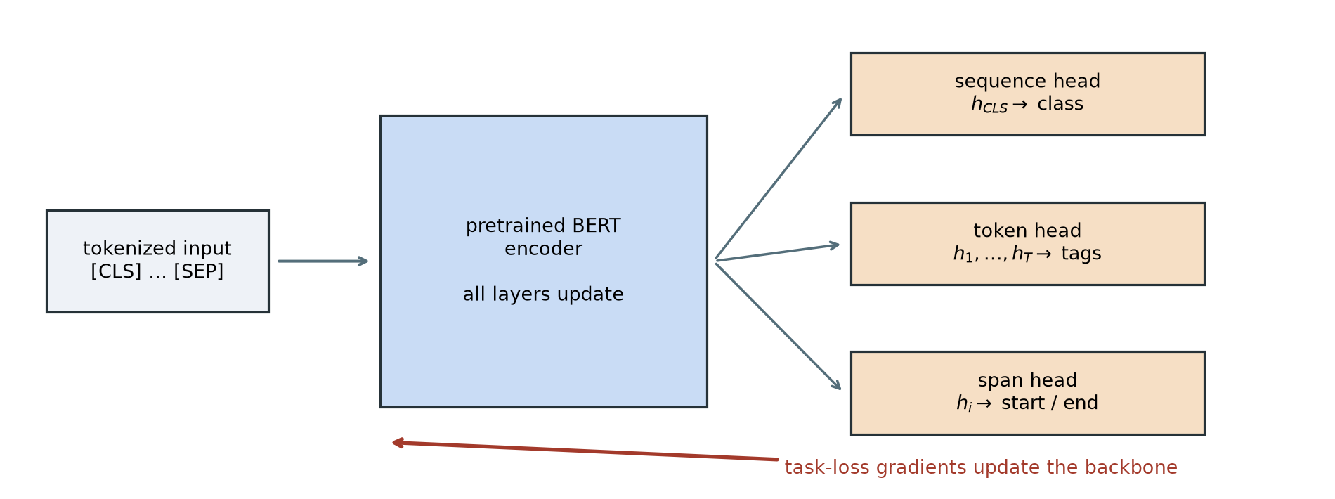
Pretraining needs a matched baseline. The scratch and pretrained arms must share labeled examples, head initialization, minibatch order, update count, evaluation, and downstream hyperparameters. The pretrained arm has already used extra compute on unlabeled data. The comparison estimates what pretraining adds, not performance at equal total compute.

18.6 A controlled transfer lab

In Chapter 10, we listed three conditions that bear on whether transfer helps: scarce target labels, a feature-hungry target task, and pretraining data that plausibly covers the target’s features at a matched scale. They are easy to state and surprisingly hard to test. A first pilot asked a tiny encoder to tell true continuations of passages in this book from segments spliced in from distant passages. The five-seed MLM gain was small, faded as labels increased, and lost decisively to a weighted lexical-overlap baseline. We rejected that task as the chapter’s affirmative experiment: this pilot did not isolate what pretraining contributed.

The replacement lab is synthetic by design, and each condition is a choice that its construction controls. The construction removes spelling, frequency, and downstream-context shortcuts so that source coverage is a controllable variable.

Build a latent regularity

We generate eighty random four-letter token strings and divide them into two latent families. Family assignment is independent of spelling. Forty covered strings (20 per family) each appear eight times in an unlabeled MLM corpus. Forty more (20 per family) live in the input vocabulary, but we withhold them from MLM input sequences, random replacements, and prediction targets.

Each covered word receives eight source sentences. Six contain cues from its own family; two deliberately contain cues from the other family. One family appears near words such as rain, soil, roots, and garden; the other appears near power, metal, gears, and workshop. The 25% cue noise gives every covered string a mixture of supporting and opposing contexts, so the family signal holds only on average.

Figure 18.4: The controlled transfer lab makes source exposure and downstream evaluation separate, auditable choices. Family is independent of spelling. Only the 40 covered types enter MLM inputs, random replacements, or targets; each contributes eight source sentences with six own-family and two cross-family cues. The neutral downstream template then separates labeled covered types, held-out covered test types, and all 40 source-invisible controls.

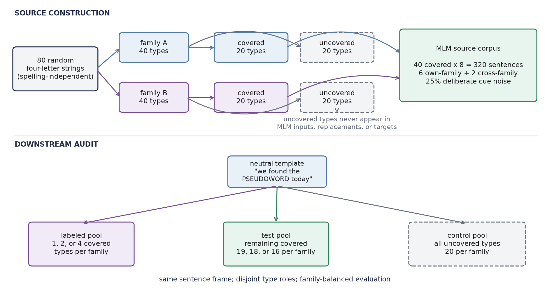
Read Figure 18.4 from top to bottom. We decide source exposure before we form the neutral downstream sentence, so the covered test pool measures transfer to covered types excluded from the downstream labeled set, and the uncovered pool audits what vocabulary membership alone can buy.

The downstream input is always the neutral, previously unseen template

\[ \text{“we found the PSEUDOWORD today.”} \]

No family cue remains. A classifier reads the generated token’s hidden state and receives only 1, 2, or 4 labeled word types from each family. We evaluate on the remaining, held-out covered types, never on the labeled types. The 40 uncovered controls use the same neutral sentence. Source and target use the same atomic token granularity and similarly short sequences, making “matched scale” explicit rather than assuming it from a shared domain.

1. Fix the lab constants, draw 80 four-letter strings, split them by family and coverage, and list eight cue pairs.
2. Define the reusable helpers: source_sentences and encode.
3. Construct the controlled source and target distributions.
4. Check the claimed identities, shapes, or invariants.
5. Print the source sentence count, vocabulary size, and covered and uncovered string counts.

# [1]
SEED = 6050
WIDTH = 48
HEADS = 4
FF_WIDTH = 96
BLOCKS = 2
MAX_LEN = 10
PRETRAIN_STEPS = 600
BATCH_SIZE = 64
LABEL_COUNTS = (1, 2, 4)
REPLICATE_SEEDS = tuple(range(6050, 6055))

torch.set_num_threads(4)
torch.use_deterministic_algorithms(True)

forms = [
    "".join(letters)
    for letters in itertools.product("bglmprstvz", "aeiou", "dknrst", "aeiou")
]
form_order = torch.randperm(
    len(forms), generator=torch.Generator().manual_seed(SEED)
)[:80]
token_strings = [forms[index] for index in form_order]
family_words = [token_strings[:40], token_strings[40:]]
covered_words = [words[:20] for words in family_words]
uncovered_words = [words[20:40] for words in family_words]

context_pairs = [
    ("rain", "power"),
    ("soil", "metal"),
    ("roots", "gears"),
    ("water", "fuel"),
    ("garden", "workshop"),
    ("grows", "moves"),
    ("blooms", "turns"),
    ("sunlight", "current"),
]

# [2]
def source_sentences(word: str, family: int) -> list[list[str]]:
    cue = [pair[family] for pair in context_pairs]
    other = [pair[1 - family] for pair in context_pairs]
    return [
        ["after", cue[0], "the", word, cue[5]],
        ["the", word, "needs", cue[3], "near", cue[1]],
        [cue[2], "support", "the", word],
        ["in", "the", cue[4], "the", word, cue[6]],
        ["we", "found", "the", word, "beside", cue[1]],
        [cue[0], "and", cue[7], "help", "the", word],
        ["the", word, "rests", "near", other[4]],
        ["today", "the", word, "follows", other[2]],
    ]

sentences: list[list[str]] = []
# [3]
for family, words in enumerate(covered_words):
    for word in words:
        sentences.extend(source_sentences(word, family))

specials = ["[PAD]", "[UNK]", "[CLS]", "[SEP]", "[MASK]"]
ordinary = sorted(
    {token for sentence in sentences for token in sentence} | set(token_strings)
)
vocabulary = specials + [token for token in ordinary if token not in specials]
stoi = {token: index for index, token in enumerate(vocabulary)}
PAD, UNK, CLS, SEP, MASK = [stoi[token] for token in specials]

def encode(sentence: list[str]) -> torch.Tensor:
    ids = [CLS] + [stoi.get(token, UNK) for token in sentence] + [SEP]
    ids += [PAD] * (MAX_LEN - len(ids))
    return torch.tensor(ids[:MAX_LEN])

source_ids = torch.stack([encode(sentence) for sentence in sentences])
uncovered_ids = torch.tensor([
    stoi[word] for family in uncovered_words for word in family
])
source_token_ids = torch.unique(source_ids)
random_pool = source_token_ids[
    ~torch.isin(source_token_ids, torch.tensor([PAD, CLS, SEP]))
]

# [4]
assert len(sentences) == 320
assert len(vocabulary) == 115
assert not torch.isin(source_ids, uncovered_ids).any()
# [5]
print(f"source: {len(sentences)} sentences; vocabulary: {len(vocabulary)} tokens")
print(f"covered/uncovered token strings: 40 / {len(uncovered_ids)}")

source: 320 sentences; vocabulary: 115 tokens
covered/uncovered token strings: 40 / 40

This is an atomic word-level vocabulary, not WordPiece. That simplification is intentional: splitting the generated strings into subwords could let spelling leak family identity. The source generator, not natural language, defines the latent regularity, so the experiment can demonstrate a mechanism but cannot estimate real-world BERT performance.

A small BERT-style encoder

The encoder has two post-LayerNorm blocks, width 48, four heads, learned absolute positions, full nonpadding attention, and GELU feedforward layers. Here \(\operatorname{GELU}(x)=x\Phi(x)\), where \(\Phi\) is the standard-normal cumulative distribution function. Original BERT used GELU, which scales each input by a smooth gate that depends on that input. The lab omits segment embeddings, NSP, and dropout. Its 43,920 encoder parameters make the study fast enough to repeat end to end, while preserving the relevant path from bidirectional attention to MLM to fine-tuning.

1. Define the reusable helpers: FullAttention, EncoderBlock, and TinyBertEncoder.
2. Define the reusable helpers: MaskedLanguageModel and corrupt.
3. Count the parameters of a freshly built TinyBertEncoder.
4. Define full attention, the encoder, and the MLM head.

# [1]
class FullAttention(nn.Module):
    def __init__(self) -> None:
        super().__init__()
        self.qkv = nn.Linear(WIDTH, 3 * WIDTH)
        self.output = nn.Linear(WIDTH, WIDTH)

    def forward(
        self, x: torch.Tensor, visible: torch.Tensor
    ) -> torch.Tensor:
        batch, length, _ = x.shape
        head_width = WIDTH // HEADS
        qkv = self.qkv(x).view(
            batch, length, 3, HEADS, head_width
        )
        q, k, v = qkv.permute(2, 0, 3, 1, 4)
        scores = q @ k.transpose(-2, -1) / head_width**0.5
        scores = scores.masked_fill(
            ~visible[:, None, None, :], float("-inf")
        )
        weights = F.softmax(scores, dim=-1)
        mixed = (weights @ v).transpose(1, 2).reshape(
            batch, length, WIDTH
        )
        return self.output(mixed)

class EncoderBlock(nn.Module):
    def __init__(self) -> None:
        super().__init__()
        self.attention = FullAttention()
        self.norm1 = nn.LayerNorm(WIDTH)
        self.ff = nn.Sequential(
            nn.Linear(WIDTH, FF_WIDTH),
            nn.GELU(),
            nn.Linear(FF_WIDTH, WIDTH),
        )
        self.norm2 = nn.LayerNorm(WIDTH)

    def forward(
        self, x: torch.Tensor, visible: torch.Tensor
    ) -> torch.Tensor:
        x = self.norm1(x + self.attention(x, visible))
        return self.norm2(x + self.ff(x))

class TinyBertEncoder(nn.Module):
    def __init__(self) -> None:
        super().__init__()
        self.token_embedding = nn.Embedding(
            len(vocabulary), WIDTH, padding_idx=PAD
        )
        self.position_embedding = nn.Embedding(MAX_LEN, WIDTH)
        self.blocks = nn.ModuleList([
            EncoderBlock() for _ in range(BLOCKS)
        ])
        nn.init.normal_(self.token_embedding.weight, std=0.02)
        nn.init.normal_(self.position_embedding.weight, std=0.02)
        with torch.no_grad():
            self.token_embedding.weight[PAD].zero_()

    def forward(self, ids: torch.Tensor) -> torch.Tensor:
        positions = torch.arange(ids.shape[1], device=ids.device)
        hidden = (
            self.token_embedding(ids)
            + self.position_embedding(positions)
        )
        visible = ids != PAD
        for block in self.blocks:
            hidden = block(hidden, visible)
        return hidden

# [2]
class MaskedLanguageModel(nn.Module):
    def __init__(self, encoder: TinyBertEncoder) -> None:
        super().__init__()
        self.encoder = encoder
        self.dense = nn.Linear(WIDTH, WIDTH)
        self.norm = nn.LayerNorm(WIDTH)
        self.decoder = nn.Linear(WIDTH, len(vocabulary))

    def forward(
        self, ids: torch.Tensor, selected: torch.Tensor
    ) -> torch.Tensor:
        hidden = self.encoder(ids)[selected]
        hidden = self.norm(F.gelu(self.dense(hidden)))
        return self.decoder(hidden)

def corrupt(
    ids: torch.Tensor,
    generator: torch.Generator,
) -> tuple[torch.Tensor, torch.Tensor, torch.Tensor]:
    eligible = (ids != PAD) & (ids != CLS) & (ids != SEP)
    selected = eligible & (
        torch.rand(ids.shape, generator=generator) < 0.15
    )
    if not selected.any():
        rows, columns = torch.where(eligible)
        choice = torch.randint(
            len(rows), (1,), generator=generator
        )
        selected[rows[choice], columns[choice]] = True

    draw = torch.rand(ids.shape, generator=generator)
    mask_sites = selected & (draw < 0.8)
    random_sites = selected & (draw >= 0.8) & (draw < 0.9)
    corrupted = ids.clone()
    corrupted[mask_sites] = MASK
    random_choices = torch.randint(
        len(random_pool), ids.shape, generator=generator
    )
    random_ids = random_pool[random_choices]
    corrupted[random_sites] = random_ids[random_sites]

    unchanged_sites = selected & ~mask_sites & ~random_sites
    counts = torch.tensor([
        mask_sites.sum().item(),
        random_sites.sum().item(),
        unchanged_sites.sum().item(),
    ])
    assert not (selected & ~eligible).any()
    assert not torch.isin(corrupted, uncovered_ids).any()
    return corrupted, selected, counts

# [3]
encoder_parameters = sum(
    parameter.numel() for parameter in TinyBertEncoder().parameters()
)
# [4]
print(f"encoder parameters: {encoder_parameters:,}")

encoder parameters: 43,920

We deliberately untie the MLM decoder from the input embedding table. The original released BERT code explicitly tied those weights, but tying would update an uncovered input row through the vocabulary softmax even when that token never appeared. The lab goes further: we draw random replacements only from source tokens, and the code later asserts that every uncovered input embedding remains bitwise unchanged through pretraining. Untied decoder rows for the controls still participate as negative softmax classes, but they are discarded downstream and never expose a control token’s context or identity to the encoder input.

Pretrain, then adapt

We save one encoder at initialization and pretrain that same encoder with MLM. The two downstream arms then receive the same labeled word types, identical classifier-head tensors, the same number of full-batch updates, and the same learning rates. We give the encoder 600 MLM updates and each downstream arm 160 full-batch updates. All encoder weights move in both arms. We run the study once for each of five seeds, and each seed repeats initialization, corruption, MLM, label selection, and fine-tuning, not merely the last classifier fit.

1. Define TensorState as shorthand for a dictionary that maps string names to tensors.
2. Define the reusable helpers: pretrain, neutral_sentence, and WordClassifier.
3. Define the reusable helpers: fit_classifier and classifier_accuracy.
4. Pretrain five paired encoders and fine-tune all weights.
5. Print selection counts and branch shares, then scratch and pretrained accuracy on each word pool per label count.

# [1]
TensorState = dict[str, torch.Tensor]

# [2]
def pretrain(
    seed: int,
) -> tuple[TensorState, TensorState, torch.Tensor, int]:
    torch.manual_seed(seed)
    encoder = TinyBertEncoder()
    initial = copy.deepcopy(encoder.state_dict())
    mlm = MaskedLanguageModel(encoder)
    optimizer = torch.optim.Adam(mlm.parameters(), lr=1e-3)
    index_generator = torch.Generator().manual_seed(seed + 1)
    mask_generator = torch.Generator().manual_seed(seed + 2)
    schedule = torch.randint(
        len(source_ids),
        (PRETRAIN_STEPS, BATCH_SIZE),
        generator=index_generator,
    )
    branch_counts = torch.zeros(3, dtype=torch.long)
    eligible_count = 0

    for indices in schedule:
        original = source_ids[indices]
        eligible_count += (
            (original != PAD) & (original != CLS) & (original != SEP)
        ).sum().item()
        corrupted, selected, counts = corrupt(
            original, mask_generator
        )
        branch_counts += counts
        logits = mlm(corrupted, selected)
        targets = original[selected]
        assert logits.shape == (targets.numel(), len(vocabulary))
        loss = F.cross_entropy(logits, targets)
        optimizer.zero_grad()
        loss.backward()
        nn.utils.clip_grad_norm_(mlm.parameters(), 1.0)
        optimizer.step()

    pretrained = copy.deepcopy(mlm.encoder.state_dict())
    initial_control = initial["token_embedding.weight"][uncovered_ids]
    final_control = pretrained["token_embedding.weight"][uncovered_ids]
    assert torch.equal(initial_control, final_control)
    return initial, pretrained, branch_counts, eligible_count

def neutral_sentence(word: str) -> torch.Tensor:
    return encode(["we", "found", "the", word, "today"])

class WordClassifier(nn.Module):
    def __init__(
        self, encoder_state: TensorState, head_state: TensorState
    ) -> None:
        super().__init__()
        self.encoder = TinyBertEncoder()
        self.encoder.load_state_dict(encoder_state)
        self.head = nn.Linear(WIDTH, 2)
        self.head.load_state_dict(head_state)

    def forward(self, ids: torch.Tensor) -> torch.Tensor:
        # [CLS] we found the WORD today [SEP] -> WORD is position 4.
        return self.head(self.encoder(ids)[:, 4])

# [3]
def fit_classifier(
    encoder_state: TensorState,
    head_state: TensorState,
    family_zero: list[str],
    family_one: list[str],
) -> tuple[WordClassifier, float]:
    inputs = torch.stack([
        neutral_sentence(word)
        for word in family_zero + family_one
    ])
    targets = torch.tensor(
        [0] * len(family_zero) + [1] * len(family_one)
    )
    model = WordClassifier(encoder_state, head_state)
    optimizer = torch.optim.Adam([
        {"params": model.encoder.parameters(), "lr": 2e-4},
        {"params": model.head.parameters(), "lr": 2e-3},
    ])
    for _ in range(160):
        loss = F.cross_entropy(model(inputs), targets)
        optimizer.zero_grad()
        loss.backward()
        optimizer.step()
    train_accuracy = (
        (model(inputs).argmax(1) == targets).float().mean().item()
    )
    return model, train_accuracy

@torch.no_grad()
def classifier_accuracy(
    model: WordClassifier,
    family_zero: list[str],
    family_one: list[str],
) -> float:
    inputs = torch.stack([
        neutral_sentence(word)
        for word in family_zero + family_one
    ])
    targets = torch.tensor(
        [0] * len(family_zero) + [1] * len(family_one)
    )
    return (
        (model(inputs).argmax(1) == targets).float().mean().item()
    )

paired_results: dict[int, list[tuple[float, float]]] = {
    count: [] for count in LABEL_COUNTS
}
uncovered_results: dict[int, list[tuple[float, float]]] = {
    count: [] for count in LABEL_COUNTS
}
training_results: dict[int, list[tuple[float, float]]] = {
    count: [] for count in LABEL_COUNTS
}
all_branches = torch.zeros(3, dtype=torch.long)
all_eligible = 0
first_states: tuple[TensorState, TensorState] | None = None

# [4]
for replicate_seed in REPLICATE_SEEDS:
    initial_state, pretrained_state, counts, eligible_count = pretrain(
        replicate_seed
    )
    if first_states is None:
        first_states = (initial_state, pretrained_state)
    all_branches += counts
    all_eligible += eligible_count

    label_generator = torch.Generator().manual_seed(replicate_seed)
    order_zero = torch.randperm(
        len(covered_words[0]), generator=label_generator
    ).tolist()
    order_one = torch.randperm(
        len(covered_words[1]), generator=label_generator
    ).tolist()
    torch.manual_seed(replicate_seed + 10_000)
    head_state = copy.deepcopy(nn.Linear(WIDTH, 2).state_dict())

    for count in LABEL_COUNTS:
        label_zero = [covered_words[0][i] for i in order_zero[:count]]
        label_one = [covered_words[1][i] for i in order_one[:count]]
        test_zero = [covered_words[0][i] for i in order_zero[count:]]
        test_one = [covered_words[1][i] for i in order_one[count:]]

        scratch, scratch_train = fit_classifier(
            initial_state, head_state, label_zero, label_one
        )
        pretrained, pretrained_train = fit_classifier(
            pretrained_state, head_state, label_zero, label_one
        )
        scratch_score = classifier_accuracy(
            scratch, test_zero, test_one
        )
        pretrained_score = classifier_accuracy(
            pretrained, test_zero, test_one
        )
        scratch_uncovered = classifier_accuracy(
            scratch, uncovered_words[0], uncovered_words[1]
        )
        pretrained_uncovered = classifier_accuracy(
            pretrained, uncovered_words[0], uncovered_words[1]
        )
        paired_results[count].append(
            (scratch_score, pretrained_score)
        )
        uncovered_results[count].append(
            (scratch_uncovered, pretrained_uncovered)
        )
        training_results[count].append(
            (scratch_train, pretrained_train)
        )

branch_shares = all_branches / all_branches.sum()
# [5]
print(
    "selected targets across five runs: "
    f"{all_branches.sum().item():,}"
)
print(f"eligible positions: {all_eligible:,}")
print(
    "realized selection rate: "
    f"{all_branches.sum().item() / all_eligible:.3%}"
)
print("realized mask/random/unchanged shares:", branch_shares.tolist())
for count in LABEL_COUNTS:
    pairs = np.array(paired_results[count])
    control_pairs = np.array(uncovered_results[count])
    train_pairs = np.array(training_results[count])
    deltas = pairs[:, 1] - pairs[:, 0]
    print(
        f"{count}/family: scratch={pairs[:, 0].mean():.3f}, "
        f"pretrained={pairs[:, 1].mean():.3f}, "
        f"delta={deltas.mean():+.3f}, wins={(deltas > 0).sum()}/5, "
        f"uncovered={control_pairs[:, 0].mean():.3f}/"
        f"{control_pairs[:, 1].mean():.3f}, "
        f"train={train_pairs[:, 0].mean():.3f}/"
        f"{train_pairs[:, 1].mean():.3f}"
    )

selected targets across five runs: 155,019
eligible positions: 1,032,096
realized selection rate: 15.020%
realized mask/random/unchanged shares: [0.8003599643707275, 0.09977486729621887, 0.09986517578363419]
1/family: scratch=0.468, pretrained=0.995, delta=+0.526, wins=5/5, uncovered=0.475/0.425, train=1.000/1.000
2/family: scratch=0.489, pretrained=1.000, delta=+0.511, wins=5/5, uncovered=0.500/0.440, train=1.000/1.000
4/family: scratch=0.494, pretrained=1.000, delta=+0.506, wins=5/5, uncovered=0.550/0.430, train=1.000/1.000

Across 1,032,096 eligible positions, the five runs select 155,019 (15.020%). The realized branches are 80.04% mask, 9.98% random, and 9.99% unchanged. (The MLM loss is Section 4.6.1’s Case 1, a mean over exactly the selected positions. The corruption policy defines the scored population, the batch mean estimates it without bias, and these counts make that denominator visible.) Both scratch and pretrained models reach 100% on their tiny labeled training sets in every run; failure to fit the labels therefore does not explain the scratch result.

What transferred?

Did pretraining organize covered representations in a way that scarce labels could reuse, or did the classifier merely learn the tiny label set? The downstream task, the uncovered controls, and the representation geometry each answer a different part.

1. Define the reusable representation_geometry helper.
2. Audit paired transfer, source coverage, and representation geometry.

# [1]
@torch.no_grad()
def representation_geometry(
    encoder_state: TensorState,
) -> tuple[float, float]:
    model = TinyBertEncoder()
    model.load_state_dict(encoder_state)
    words = covered_words[0] + covered_words[1]
    vectors = model(torch.stack([
        neutral_sentence(word) for word in words
    ]))[:, 4]
    vectors = vectors - vectors.mean(dim=0, keepdim=True)
    vectors = F.normalize(vectors, dim=1)
    similarities = vectors @ vectors.T
    labels = torch.tensor(
        [0] * len(covered_words[0]) + [1] * len(covered_words[1])
    )
    off_diagonal = ~torch.eye(len(words), dtype=torch.bool)
    within = similarities[
        (labels[:, None] == labels[None, :]) & off_diagonal
    ]
    between = similarities[labels[:, None] != labels[None, :]]
    return within.mean().item(), between.mean().item()

assert first_states is not None
initial_geometry = representation_geometry(first_states[0])
pretrained_geometry = representation_geometry(first_states[1])

budgets = np.array(LABEL_COUNTS)
scratch_means = np.array([
    np.mean(paired_results[count], axis=0)[0]
    for count in LABEL_COUNTS
])
pretrained_means = np.array([
    np.mean(paired_results[count], axis=0)[1]
    for count in LABEL_COUNTS
])
scratch_uncovered_means = np.array([
    np.mean(uncovered_results[count], axis=0)[0]
    for count in LABEL_COUNTS
])
pretrained_uncovered_means = np.array([
    np.mean(uncovered_results[count], axis=0)[1]
    for count in LABEL_COUNTS
])

# [2]
print(f"initial within/between: {initial_geometry}")
print(f"after MLM within/between: {pretrained_geometry}")

initial within/between: (-0.03466804325580597, -0.0160280279815197)
after MLM within/between: (0.5322557687759399, -0.5517237186431885)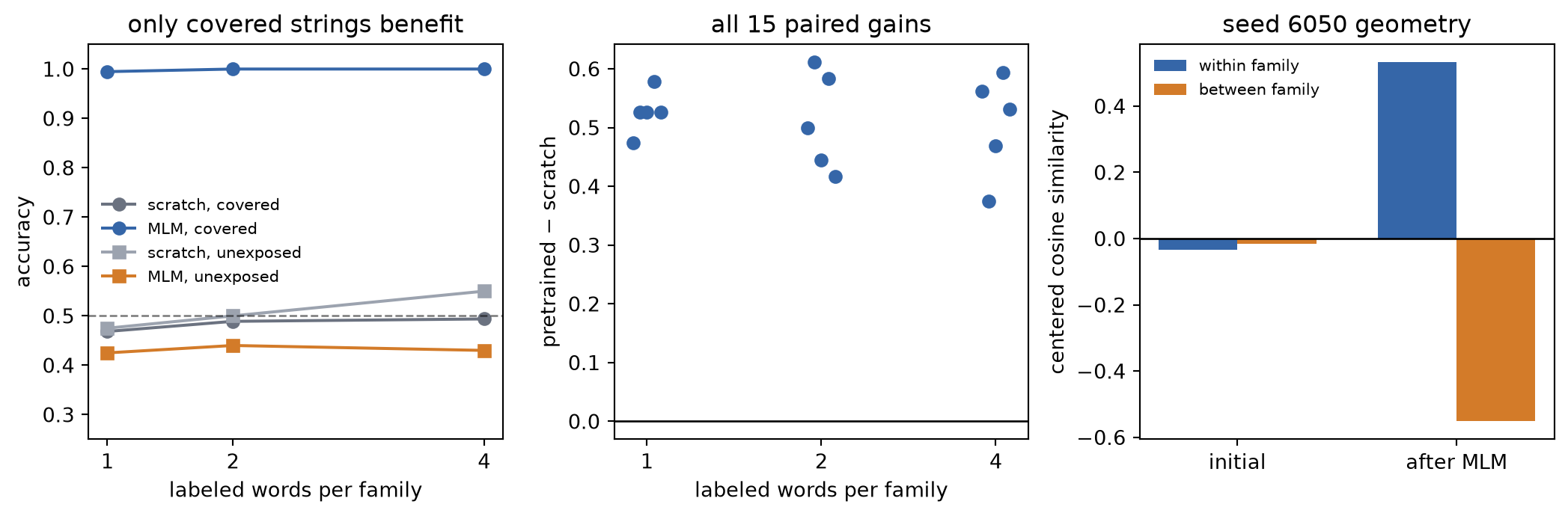

Figure 18.5: Five paired end-to-end seeds in the synthetic transfer lab. MLM initialization separates covered latent families and improves every covered-type comparison (left and center); both arms stay near chance on input-vocabulary controls withheld from MLM inputs, replacements, and targets (left). Centered cosine similarity is a representation diagnostic, not a task metric (right).

Labels / family	Scratch, covered	MLM, covered	Gain	Scratch, unexposed	MLM, unexposed
1	0.468	0.995	+0.526	0.475	0.425
2	0.489	1.000	+0.511	0.500	0.440
4	0.494	1.000	+0.506	0.550	0.430

MLM initialization wins all 15 paired covered-type comparisons. At two labels per family, for example, mean covered accuracy moves from 0.489 to 1.000. On the 40 unexposed controls, scratch and MLM-initialized means stay around chance at every budget. MLM therefore helps types whose source contexts contain the latent regularity, not arbitrary rows that merely exist in the input vocabulary.

Within each seed, larger label budgets add word types to the labeled training set and remove those same types from the test pool. The within-budget scratch-versus-MLM comparison is exact; movement across budgets is not a controlled learning curve.

The representation diagnostic agrees with the task result. In the seed chosen for the geometry, mean centered cosine similarity starts at \(-0.0347\) within a family and \(-0.0160\) between families: no useful separation. After MLM, it is \(0.5323\) within and \(-0.5517\) between. Centered cosine first subtracts the mean representation, then unit-normalizes each vector and takes a dot product: a positive value means two centered vectors point in similar directions, a negative value that they point in opposing directions. Pretraining has organized neutral-context token states around the latent source regularity, and a few labels recover that organization for covered types excluded from the downstream labeled set.

At toy scale, the construction controls each of the three conditions from Chapter 10:

• Scarce labels: the task supplies only 2, 4, or 8 labeled words total.
• A feature-hungry target: spelling, frequency, and task-context cues are neutralized; the label must transfer through the token representation.
• Source coverage at a matched scale: the generator decides which strings MLM sees, and source and target use atomic tokens and similarly short sequences. Covered strings transfer, while the uncovered strings, balanced across families and withheld from MLM inputs, replacements, and targets, remain near chance in both arms.

The result is an existence proof for a mechanism. A co-occurrence method could also recover the synthetic families; the experiment does not establish Transformer superiority. Three limits remain: the data generator builds the regularity, the pretrained arm receives extra compute, and five toy seeds do not estimate natural-language performance. The conclusion is narrower: in this controlled construction and across five seeds, MLM initialization lets a few labels recover a latent regularity for covered types excluded from the downstream labeled set; in one seed, MLM organizes covered token representations around that regularity.

18.7 Three pretraining families

Pretraining is a regime, not an architecture. The visibility rule and pretraining objective determine what a model can learn, and how it will later be used.

Table 18.3: Three pretraining families separate visibility, objective, and characteristic use.

Family	Visibility during pretraining	Objective	Characteristic use
BERT-style encoder	Full nonpadding context	Predict selected original tokens after 80/10/10 treatment	Contextual representations and task heads
GPT-style decoder	Causal prefix	Predict the next token	Autoregressive generation and adaptation
T5-style encoder–decoder	Full encoder; causal decoder with cross-attention	Generate removed spans separated by sentinel tokens	Text-to-text conditional generation

The visibility column becomes concrete in Figure 18.6. Each matrix uses queries as rows and keys as columns, exactly as in Figure 18.1.

Figure 18.6: Three pretraining families differ first in what each position may retrieve. A BERT-style encoder has full nonpadding self-attention; a GPT-style decoder has causal self-attention. T5 uses three routes in two stacks: full encoder self-attention, causal decoder self-attention, and decoder-to-encoder cross-attention. The combined T5 block summarizes the visibility of those separate sublayers; it is not one mask applied by the implementation.

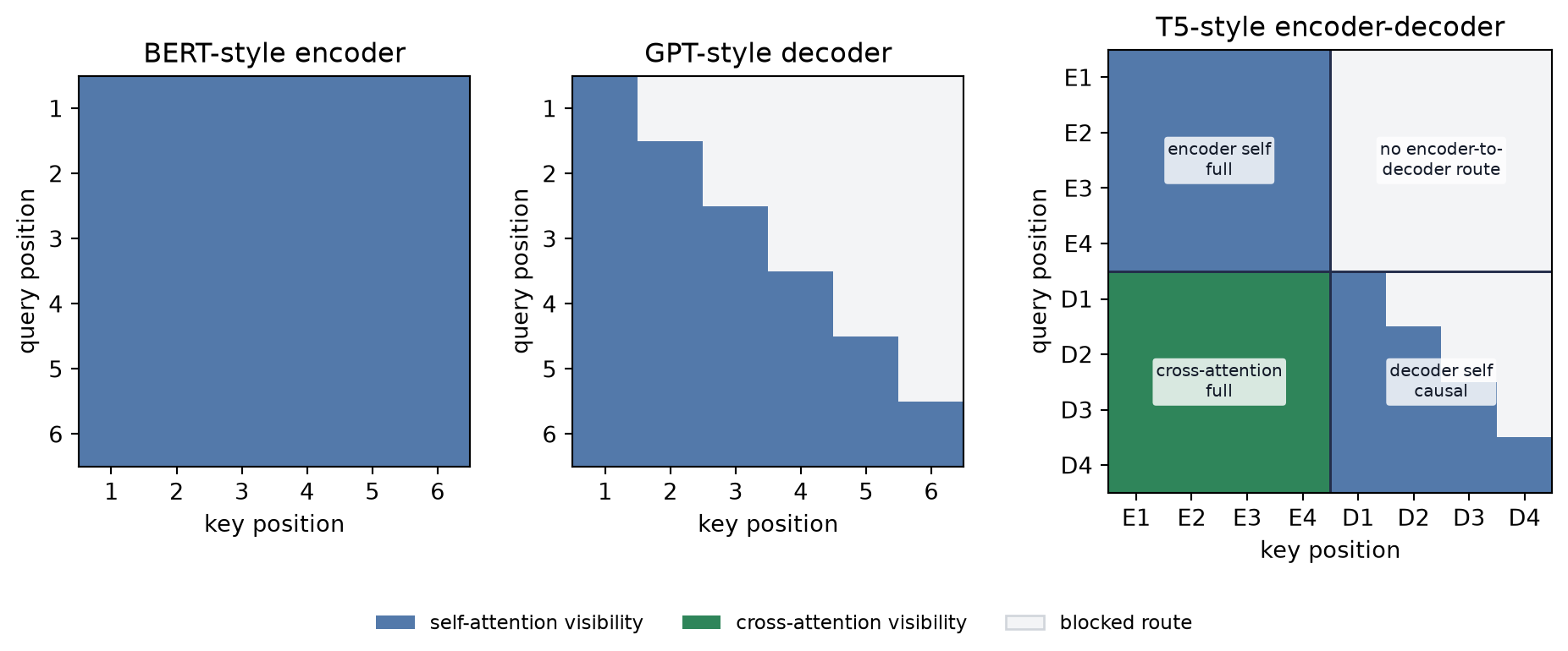
The separation in Table 18.3 matters during execution too. A GPT-style decoder can train all next-token positions in parallel under teacher forcing because the causal mask exposes only each prefix. Generation is still sequential: the model must emit a token before that token can join the next prefix. Training and inference share a factorization and visibility rule, not an execution schedule.

Once those next-token logits exist, Chapter 13’s greedy and beam-search machinery can rank continuations; the architecture changes, but decoding remains a separate decision. Chapter 20 will return to how prompts alter the context supplied to that decoder.

T5 turns tasks into text-to-text problems and marks removed spans with learned sentinel tokens. Its encoder produces a sequence of memory states under full visibility; its causal decoder cross-attends to that sequence while generating the target. It does not squeeze the input into one fixed bottleneck vector. These families trade representation, generation, and input–output structure differently; they are not a ranking from old to new.

18.8 What changed after 2018

Before the pretrained era, a new labeled dataset often implied a new model trained from a random initialization. After BERT and its contemporaries, the default question changed: which pretrained model, which adaptation, and which data interface fit the task?

Three consequences follow.

Optimization starts elsewhere. The downstream run begins in a parameter region already shaped by a broad source objective. The task is not asking a few labels to invent syntax and semantics from scratch.

Data work moves upstream. Corpus choice, tokenization, corruption, and source coverage become part of model design. Pretraining is curriculum at dataset scale.

One backbone serves many interfaces. A sequence head, token head, or span head can reuse the same encoder. That modularity makes comparison easier, but also makes pretraining assumptions easy to inherit without inspecting them.

The regime introduces new failure modes. Source bias can transfer with useful features. A vocabulary can represent a token without supplying useful exposure. Full fine-tuning can forget source behavior or become too expensive as the backbone grows.

A learned summary token can gather image patches instead of words; Chapter 19 moves the encoder from text to images and asks what scaling changes. Fine-tuning changed every encoder weight here; Chapter 20 asks what adaptation remains when most, or all, of those weights must stay fixed.

NoteCheck yourself

Close the book for one minute and reconstruct masked-language-model pretraining.

• How are visibility, supervision, corruption, and padding represented separately?
• Why is the 80/10/10 rule conditional on selection?
• What changes between a frozen probe and full fine-tuning?

18.9 Okay, so: pretraining manufactures supervision

1. Visibility, selection, corruption, and padding are separate. BERT removes the causal triangle, selects loss targets, then applies the 80/10/10 treatment so copying cannot solve most of them. [MASK] is a token, not an attention ban.
2. MLM turns raw text into supervision. Select 15% of eligible positions; conditional on selection, use 80% mask, 10% random, and 10% unchanged. All selected positions predict their original tokens.
3. BERT is a full-context Transformer encoder. WordPiece tokens, learned token/position/segment embeddings, post-LayerNorm blocks, MLM, and historical NSP define the original recipe.
4. Fine-tuning updates the encoder. Training only a new head over frozen features is a probe. Standard BERT adaptation moves the pretrained backbone and task head together.
5. In the toy lab, transfer reaches only the covered types. Across five full seeds, MLM initialization wins every covered-type comparison under 2–8 total labels; input-vocabulary controls withheld from MLM inputs, replacements, and targets remain near chance in both arms.
6. Pretraining changed the unit of work. The field moved from one random model per task toward reusable backbones and specialized adaptation. Corpus, objective, visibility, and adaptation now belong to one design decision.

Sources and further reading

• Peters et al., Deep Contextualized Word Representations: ELMo and fixed contextual features from forward and backward language models.
• Howard and Ruder, Universal Language Model Fine-tuning for Text Classification: ULMFiT’s full-model adaptation recipe.
• Radford et al., Improving Language Understanding by Generative Pre-Training: causal Transformer pretraining followed by supervised adaptation.
• Sennrich, Haddow, and Birch, Neural Machine Translation of Rare Words with Subword Units: the frequency-driven BPE adaptation for subword vocabularies.
• Devlin et al., BERT: Pre-training of Deep Bidirectional Transformers for Language Understanding: the original BERT architecture, MLM/NSP objectives, and fine-tuning results.
• Google Research, BERT pretraining implementation: the released implementation documents the tied input/output embedding weights.
• Liu et al., RoBERTa: A Robustly Optimized BERT Pretraining Approach: a later study of BERT training choices, including removal of NSP.
• Raffel et al., Exploring the Limits of Transfer Learning with a Unified Text-to-Text Transformer: the T5 text-to-text framework and span-corruption recipe.
• Salazar et al., Masked Language Model Scoring (2020): token-by-token masking as a pseudo-log-likelihood sentence score, with the distinction between a score and a normalized left-to-right likelihood.

Exercises

1. (Pencil.) For [CLS] the wug is calm [SEP] [PAD] [PAD], suppose wug is selected and replaced by [MASK]. Draw Chapter 16’s causal visibility matrix and BERT’s full nonpadding visibility matrix, using queries as rows and keys as columns. Separately mark the one position that contributes MLM loss. Why may neighboring tokens attend to [MASK], and why would full visibility leak information in a next-token generator?
2. (Pencil.) A batch contains 2,000 eligible ordinary tokens. Under BERT’s policy, how many positions are expected to be selected, replaced by [MASK], replaced by a random token, and left unchanged? How many contribute direct MLM loss? Explain why 12% is not the supervision rate.
3. (Code.) For token IDs \((B,T)\), width \(d\), and vocabulary size \(|V|\), add assertions for hidden states \((B,T,d)\), dense logits \((B,T,|V|)\), selected logits \((|M|,|V|)\), and selected targets \((|M|,)\). Assert that [PAD], [CLS], and [SEP] are never selected. Show numerically that selected-only cross-entropy matches dense cross-entropy when unselected targets use ignore_index.
4. (Code.) Starting from the same pretrained checkpoint and split, compare a frozen encoder probe with full fine-tuning in the generated-token lab. Match head tensors, labeled types, updates, and seeds. Plot all five paired results rather than only their means. Which regime wins here, and what broader claim would outrun the experiment?
5. (Audit.) Reproduce paired gains for covered and control strings at all three label budgets. Map the evidence to the three transfer conditions from Chapter 10. Explain the assertion that uncovered input embeddings stay bitwise unchanged, name two unsupported conclusions, and propose one predeclared coverage test.
6. (Pencil.) Define the pseudo-log-likelihood \(\operatorname{PLL}(x)=\sum_{i=1}^{T}\log p(x_i\mid x_{\setminus i})\) and explain why ordinary masked scoring costs \(T\) forward passes. Show why the collection of conditionals need not define one normalized joint distribution. (Code.) Score minimal sentence pairs from the controlled lab by masking each ordinary token once. Train a small causal model on that same corpus and vocabulary with Chapter 12’s trainer, then compare rankings under one declared length convention. Assert that special and padding tokens contribute neither PLL score nor mask position. Report PLL as a score, not a normalized sentence likelihood.