11  The Gradient Has a Memory: Reverse Accumulation and Checkpointing

NS · Numerical stability Geometric quiet · Dynamic supporting · Algorithmic primary

Take the scalar computation

\[ a=xy,\qquad b=a+x,\qquad c=ay,\qquad L=bc \tag{11.1}\]

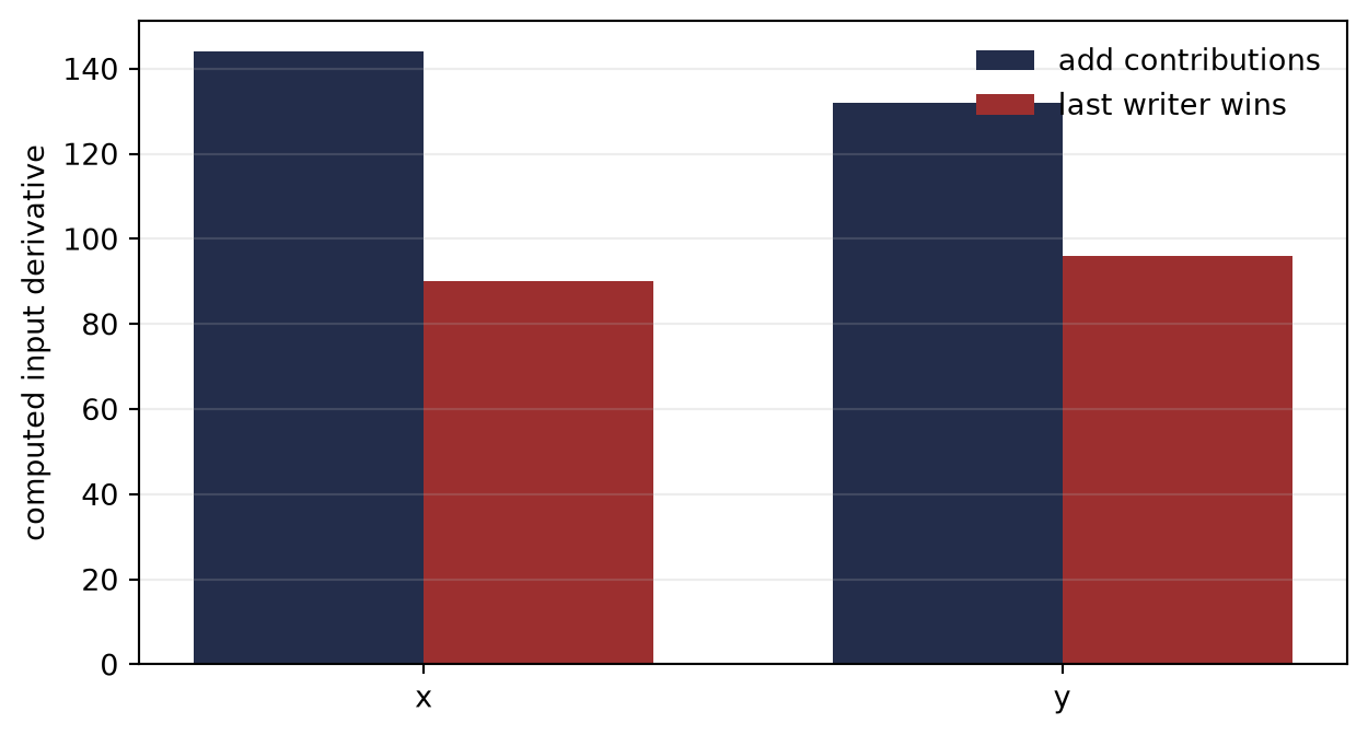
at \(x=2\) and \(y=3\). The intermediate \(a\) feeds two children. On the reverse sweep, one path contributes \(18\) to the cotangent of \(a\) and the other contributes \(24\). The correct value is their sum, \(42\).

An implementation that stores only the last contribution returns

\[ \frac{\partial L}{\partial x}=90,\qquad \frac{\partial L}{\partial y}=96, \]

instead of the correct \((144,132)\). Every local derivative can be correct while the total gradient is wrong.

ImportantPrediction

What must a reverse derivative engine remember: graph structure, numerical values, path contributions, or all three?

11.1 One node, two debts

The sibling volume owns the mechanics of the chain rule and the construction of a tiny reverse derivative engine. Its backpropagation chapter is the recap if those mechanics are unfamiliar. This chapter owns a different question: once the computation is a directed acyclic graph, what does a correct reverse sweep accumulate, retain, and recompute?

1. Load the chapter-pinned reverse-accumulation instruments.
2. Encode the fan-out computation as a scalar tape.
3. Run a correct additive reverse accumulation.
4. Run the named wrong implementation that overwrites cotangents.
5. Inspect the two path contributions into the shared node.
6. Compare the resulting input derivatives.

import matplotlib.pyplot as plt
import numpy as np

# [1]

from trainable_harness import TapeNode, reverse_accumulate

# [2]
x, y = 2.0, 3.0
tape = [
    TapeNode(x),
    TapeNode(y),
    TapeNode(x * y, ((0, y), (1, x))),
    TapeNode(x * y + x, ((2, 1.0), (0, 1.0))),
    TapeNode(x * y * y, ((2, y), (1, x * y))),
    TapeNode(
        (x * y + x) * (x * y * y),
        ((3, x * y * y), (4, x * y + x)),
    ),
]

# [3]
correct = reverse_accumulate(tape)

# [4]
def overwrite_shared_node(nodes, shared_index, reverse_order):
    cotangents = np.zeros(len(nodes), dtype=np.float64)
    cotangents[-1] = 1.0
    for node_index in reverse_order:
        incoming = cotangents[node_index]
        for parent_index, local_derivative in nodes[node_index].parents:
            contribution = incoming * local_derivative
            if parent_index == shared_index:
                cotangents[parent_index] = contribution
            else:
                cotangents[parent_index] += contribution
    return cotangents

overwrite = overwrite_shared_node(
    tape,
    shared_index=2,
    reverse_order=(5, 3, 4, 2, 1, 0),
)

# [5]
contributions = [correct[3], correct[4] * y]
assert np.allclose(contributions, [18.0, 24.0])
assert np.allclose(correct[:2], [144.0, 132.0])

# [6]
labels = ["x", "y"]
positions = np.arange(len(labels))
width = 0.36
fig, axis = plt.subplots(figsize=(6.6, 3.6))
axis.bar(
    positions - width / 2,
    correct[:2],
    width,
    label="add contributions",
    color="#232D4B",
)
axis.bar(
    positions + width / 2,
    overwrite[:2],
    width,
    label="last writer wins",
    color="#9C2F2F",
)
axis.set(
    xticks=positions,
    xticklabels=labels,
    ylabel="computed input derivative",
)
axis.grid(axis="y", alpha=0.22)
axis.legend(frameon=False)
plt.tight_layout()
plt.show()

print(f"harness={manifest['harness_ref']} wheel={manifest['wheel_sha256'][:12]}")
print(f"contributions into a={contributions}; accumulated={correct[2]}")
print(f"correct: dx={correct[0]:.1f}, dy={correct[1]:.1f}")
print(f"overwrite: dx={overwrite[0]:.1f}, dy={overwrite[1]:.1f}")

Figure 11.1: A reverse sweep must add all downstream contributions at a fan-out node. Overwriting the cotangent of the shared intermediate a loses one path and produces incorrect derivatives even though every local derivative rule is correct.

harness=ch-11 wheel=c9e645efbb2e
contributions into a=[np.float64(18.0), np.float64(24.0)]; accumulated=42.0
correct: dx=144.0, dy=132.0
overwrite: dx=90.0, dy=96.0

The word backward can hide this obligation. A graph is not necessarily a chain. Reverse accumulation solves a conservation problem: every downstream use creates a derivative debt to its parent, and all debts must be paid before that parent propagates further.

The defective sweep visits the incomparable siblings \(b\) and \(c\) in that order, so the \(c\) path becomes the last writer at \(a\). Reversing the sibling order produces a different wrong gradient. The bug is therefore sensitive to an implementation detail the derivative should not depend on.

11.2 One derivative, two orientations

Let \(F:\mathbb{R}^n\to\mathbb{R}^m\) and let \(\matr{J}_F(\vect{x})\in\mathbb{R}^{m\times n}\) be its Jacobian. Two matrix-vector products expose two computational orientations:

\[ \underbrace{\matr{J}_F(\vect{x})\vect{v}}_{\text{JVP}} \in\mathbb{R}^{m}, \qquad \underbrace{\vect{u}^{\mathsf T}\matr{J}_F(\vect{x})}_{\text{VJP}} \in\mathbb{R}^{n}. \tag{11.2}\]

A Jacobian–vector product propagates an input perturbation forward. A vector–Jacobian product propagates an output cotangent backward.

Theorem 11.1 (Sweep counts follow Jacobian orientation) Suppose one forward-mode sweep computes \(\matr{J}_F(\vect{x})\vect{v}\) and one reverse-mode sweep computes \(\vect{u}^{\mathsf T}\matr{J}_F(\vect{x})\). Reconstructing the full Jacobian from basis directions requires \(n\) forward sweeps or \(m\) reverse sweeps. For scalar output, \(m=1\), one reverse sweep returns the full gradient.

Proof

Applying a JVP to the input basis vector \(\vect{e}_j\) returns column \(j\) of the Jacobian, so all \(n\) columns require \(n\) sweeps. Applying a VJP to the output basis vector \(\vect{e}_i\) returns row \(i\), so all \(m\) rows require \(m\) sweeps. When \(m=1\), the single row is \(\nabla F(\vect{x})^{\mathsf T}\). \(\square\)

This is an orientation result, not the slogan “reverse is always better.” When inputs are few and outputs are many, forward mode can be the cheaper choice. Scalar training objectives create the opposite geometry.

11.3 The reverse rule on a graph

Let node \(v\) store a value \(z_v\). Each edge \(v\to w\) carries the local derivative \(\partial z_w/\partial z_v\). For scalar output \(L\), define the cotangent

\[ \bar z_v:=\frac{\partial L}{\partial z_v}. \]

The graph chain rule is

\[ \bar z_v = \sum_{w\in\operatorname{children}(v)} \bar z_w \frac{\partial z_w}{\partial z_v}. \tag{11.3}\]

Theorem 11.2 (Reverse accumulation on a directed acyclic graph) Process the nodes of a scalar-output directed acyclic computation in reverse topological order. Initialize the output cotangent to one and every other cotangent to zero. For every edge \(v\to w\), add

\[ \bar z_w\frac{\partial z_w}{\partial z_v} \]

to \(\bar z_v\). After the sweep, \(\bar z_v=\partial L/\partial z_v\) at every node.

Proof

Proceed by reverse topological induction. The output node is correct by initialization. Suppose every child \(w\) of \(v\) already holds \(\bar z_w=\partial L/\partial z_w\). Every directed path from \(v\) to the output begins with exactly one edge \(v\to w\). Grouping the ordinary multivariable chain rule by that first edge gives

\[ \frac{\partial L}{\partial z_v} = \sum_w \frac{\partial L}{\partial z_w} \frac{\partial z_w}{\partial z_v}. \]

The additive updates compute precisely this sum. Reverse topological order ensures that all child cotangents are final before \(v\) is propagated. \(\square\)

WarningNamed wrong answer: last writer wins

Assignment is valid only when a node has one downstream path. At fan-out, the graph chain rule is a sum. An overwrite implementation can pass every chain-shaped test and fail on the first branch.

11.4 Instructions are cheap; saved values are not

A reverse rule often needs primal values from the forward execution. Multiplication needs the other operand. A nonlinear primitive may need its input, its output, or auxiliary statistics. The reverse program therefore has two distinct kinds of memory:

Retained object	Why it exists	Typical scale
graph or tape instructions	identify parents and local reverse rules	number of executed primitives
primal states	evaluate those reverse rules later	activation volume
cotangent buffers	accumulate downstream contributions	live differentiated values
stateful metadata	replay randomness, normalization state, or control flow	operation dependent

The tape can be compact while the saved numerical states dominate memory. This is why “reverse mode has constant-factor arithmetic overhead” does not mean “reverse mode is memory-free.” The algebraic complexity result of Baur and Strassen (1983) and the implementation survey of Baydin et al. (2018) answer the former question; training systems must also answer the latter.

11.5 Trade retained states for replay

Consider a depth-\(L\) chain. Storing every intermediate requires \(L+1\) primal states. A simple uniform checkpoint schedule chooses a block length \(k\): retain the input to every block during the forward pass, then replay each block during the reverse pass.

Theorem 11.3 (Uniform checkpoint count) If \(k\) divides \(L\), a uniform block schedule can execute reverse accumulation with peak primal-state count

\[ M(k)=\frac{L}{k}+k \tag{11.4}\]

and exactly

\[ R(k)=L-\frac{L}{k} \tag{11.5}\]

additional forward primitive evaluations. The continuous minimizer of \(M(k)\) is \(k=\sqrt L\), giving peak state \(2\sqrt L\).

Proof

The forward pass retains one state at each of the \(L/k\) block boundaries. During reverse execution of one block, at most \(k\) within-block states are materialized, so the peak is their sum. Within each block, the boundary state already exists and the remaining \(k-1\) forward transitions must be replayed. Across \(L/k\) blocks, this costs \((L/k)(k-1)=L-L/k\). Finally,

\[ \frac{L}{k}+k\ge2\sqrt L \]

by the arithmetic–geometric mean inequality, with equality at \(k=\sqrt L\). \(\square\)

The theorem is a count model. It does not claim that every state has equal size, every primitive has equal cost, or the measured wall-clock optimum is exactly \(\sqrt L\).

1. Reuse the verified C11 harness.
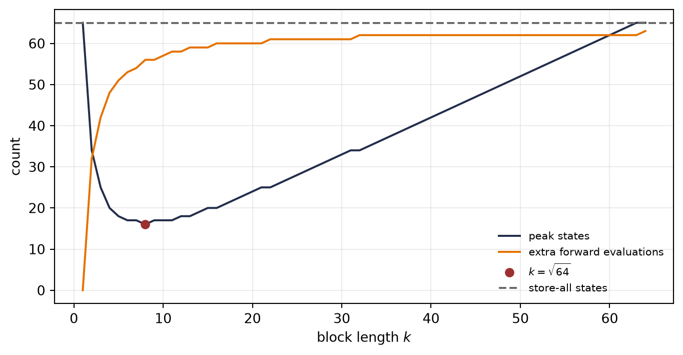
2. Enumerate all integer block lengths for a depth-64 chain.
3. Compute peak retained states and additional forward work.
4. Mark the square-root schedule.
5. Compare it with the store-all baseline.

from trainable_harness import uniform_checkpoint_cost

# [1]
assert manifest["harness_ref"] == "ch-11"

# [2]
depth = 64
block_lengths = np.arange(1, depth + 1)

# [3]
costs = [uniform_checkpoint_cost(depth, int(k)) for k in block_lengths]
peak_states = np.array([cost.peak_state_units for cost in costs])
extra_forwards = np.array([
    cost.recomputed_forward_evaluations for cost in costs
])

# [4]
chosen = uniform_checkpoint_cost(depth, 8)
assert chosen.peak_state_units == 16
assert chosen.recomputed_forward_evaluations == 56

# [5]
fig, axis = plt.subplots(figsize=(7.2, 3.8))
axis.plot(block_lengths, peak_states, color="#232D4B", label="peak states")
axis.plot(
    block_lengths, extra_forwards,
    color="#E57200", label="extra forward evaluations",
)
axis.scatter([8], [16], color="#9C2F2F", zorder=3, label="$k=\sqrt{64}$")
axis.axhline(65, color="#6b6b6b", linestyle="--", label="store-all states")
axis.set(xlabel="block length $k$", ylabel="count")
axis.grid(alpha=0.22)
axis.legend(frameon=False, fontsize=8)
plt.tight_layout()
plt.show()

print(
    f"depth={depth}; block={chosen.block_size}; "
    f"peak_states={chosen.peak_state_units}; "
    f"extra_forwards={chosen.recomputed_forward_evaluations}; "
    f"store_all={depth + 1}"
)

Figure 11.2: Uniform checkpointing trades retained primal states for forward replay in a depth-64 chain. The square-root block length k=8 reduces the count-model peak from 65 store-all states to 16 states while adding 56 forward primitive evaluations.

depth=64; block=8; peak_states=16; extra_forwards=56; store_all=65

The square-root checkpoint schedule originates in reverse-AD memory analysis by Griewank (1992) and is developed systematically by Griewank and Walther (2008). Chen et al. (2016) reintroduced the trade in the deep-learning systems setting. More elaborate schedules improve it for particular graphs and budgets. The invariant remains: discarded primal state must be reconstructed somehow.

11.6 Replay is part of the numerical contract

Recomputation sounds exact only in real arithmetic and for pure functions. On a machine, a checkpoint boundary must declare:

• the floating-point format and accumulation mode used on replay;
• random-number state for stochastic primitives;
• mutable running statistics and other stateful updates;
• control-flow decisions whose predicates depend on rounded values.

Reverse accumulation avoids the perturb-and-subtract cancellation of finite differences, but it does not escape floating-point reduction. Cotangents from many children are still summed, and their order can change the result. The reduction-order lesson from C02 has returned inside the gradient engine.

TipField note: a gradient-memory claim

Ask four questions. What values are retained? What values are replayed? What state makes replay deterministic? Is the reported saving a count model, allocated bytes, or measured peak device memory?

Three tempting escape routes do not solve the problem:

• Numerical differentiation estimates derivatives by perturbation; it is not exact and pays cancellation plus repeated evaluations.
• Symbolic differentiation can preserve graph reuse; expression explosion is not inevitable if common subexpressions remain shared.
• Reverse accumulation is not always the cheapest orientation; its advantage follows from the input/output dimensions of the derivative query.

11.7 The next diagnostic object

The reverse sweep applies transposed local Jacobians repeatedly. That tells us how a gradient is assembled, but not how the gradient changes when parameters move. C12 will differentiate the gradient action itself, using Hessian–vector products to probe curvature without materializing a dense Hessian. Later, the same product-of-local-Jacobians view will diagnose why depth can preserve, shrink, or amplify signals.

NoteCheck yourself

Suppose \(F:\mathbb{R}^{1000}\to\mathbb{R}^{4}\). How many basis sweeps are needed to materialize its Jacobian using forward mode and reverse mode? If the objective is the sum of the four outputs, how many reverse sweeps are needed for its gradient with respect to the input?

11.8 Okay, so —

• Inherited: the local chain rule and primitive reverse rules belong to the sibling volume.
• Changed: a chain-rule story became a graph accumulation and liveness problem.
• Instrumented: a one-line overwrite defect lost one of two cotangent paths; a depth-64 schedule exposed the state–replay trade.
• Established: reverse mode is efficient for scalar outputs because of Jacobian orientation, and correct DAG execution requires additive cotangents plus retained or recomputable primal state.
• Unresolved: Which curvature object should be probed before a spectrum is interpreted, and can its action be computed without materializing it?

11.9 Sources and further reading

The first published reverse-accumulation account is Linnainmaa (1970); the modern taxonomy and implementation vocabulary follow Baydin et al. (2018). The algebraic complexity boundary for derivative evaluation is due to Baur and Strassen (1983). The square-root checkpoint trade originates with Griewank (1992) and is treated in book form by Griewank and Walther (2008); Chen et al. (2016) is the deep-learning-era rediscovery and systems translation.

Reading order. Start with Baydin et al. (2018) for the JVP/VJP taxonomy, use Griewank and Walther (2008) for checkpointing and priority, then separate Baur and Strassen (1983)’s arithmetic result from Chen et al. (2016)’s systems setting.

11.10 Exercises

1. (Pencil.) Add a third child \(d=a^2\) to Equation 11.1 and replace the objective by \(L=bc+d\). Compute all three contributions into \(\bar a\) before computing the input gradients.
2. (Code.) Implement a finite-difference check of the opening gradient in binary32. Sweep the perturbation over powers of two and separate truncation error from cancellation.
3. (Code.) For depths from \(16\) to \(4096\), find the best integer uniform block length under Equation 11.4. Compare it with \(\sqrt L\) and report both peak states and replay counts.
4. (Audit.) Paper audit: Complete the Mathematical object, Evidence culture and interface, Numerical and hardware contract, Discriminating control, and Transfer verdict fields of the Paper Autopsy Protocol for one memory-efficient training paper. Mark which graph class it assumes, whether memory means saved activations or measured device allocation, whether stochastic replay is specified, and whether arithmetic count is confused with wall-clock speed.
5. (Code.) Implement replay for a chain containing one stateful random operation. Compare saved-state and recomputed derivatives under matched and unmatched random streams. Report arithmetic work, peak state, and the first derivative mismatch separately.

Baur, Walter, and Volker Strassen. 1983. “The Complexity of Partial Derivatives.” Theoretical Computer Science 22 (3): 317–30. https://doi.org/10.1016/0304-3975(83)90110-X.

Baydin, Atilim Gunes, Barak A. Pearlmutter, Alexey Andreyevich Radul, and Jeffrey Mark Siskind. 2018. “Automatic Differentiation in Machine Learning: A Survey.” Journal of Machine Learning Research 18 (153): 1–43. https://www.jmlr.org/papers/v18/17-468.html.

Chen, Tianqi, Bing Xu, Chiyuan Zhang, and Carlos Guestrin. 2016. Training Deep Nets with Sublinear Memory Cost. https://doi.org/10.48550/arXiv.1604.06174.

Griewank, Andreas. 1992. “Achieving Logarithmic Growth of Temporal and Spatial Complexity in Reverse Automatic Differentiation.” Optimization Methods and Software 1 (1): 35–54. https://doi.org/10.1080/10556789208805505.

Griewank, Andreas, and Andrea Walther. 2008. Evaluating Derivatives: Principles and Techniques of Algorithmic Differentiation. 2nd ed. Society for Industrial; Applied Mathematics. https://doi.org/10.1137/1.9780898717761.

Linnainmaa, Seppo. 1970. “The Representation of the Cumulative Rounding Error of an Algorithm as a Taylor Expansion of the Local Rounding Errors.” Master’s thesis, University of Helsinki. https://kansalliskirjasto.finna.fi/Record/helka.9933382303506253.