14 Critical on Average, Broken by Direction: Initialization and Dynamical Isometry

14.1 Criticality is a recursion with assumptions

Consider a wide coordinate

\[ h_i^{(\ell+1)}=\phi\!\left(\sum_{j=1}^{n} W_{ij}^{(\ell+1)}h_j^{(\ell)}+b_i^{(\ell+1)}\right), \tag{14.1}\]

with independent mean-zero weights of variance \(\sigma_w^2/n\). Under the usual wide, exchangeable, self-averaging approximation, a typical preactivation is approximately Gaussian and the second moment follows a scalar map.

Theorem 14.1 (Wide-model second-moment recursion) Under the independence and Gaussian-limit assumptions above,

\[ q_{\ell+1}=\sigma_w^2\, \E\!\left[\phi(\sqrt{q_\ell}Z)^2\right]+\sigma_b^2, \qquad Z\sim\mathcal N(0,1). \tag{14.2}\]

For zero-bias ReLU coordinates, \(q_{\ell+1}=\sigma_w^2q_\ell/2\); the variance-critical scale is \(\sigma_w^2=2\).

Diagnostic proof

Condition on the previous coordinates. Independence and the \(1/n\) scaling make the preactivation variance the empirical second moment times \(\sigma_w^2\), plus bias variance. The wide limit replaces that empirical moment by \(q_\ell\). Symmetry gives \(\E[\max(0,\sqrt q Z)^2]=q/2\).

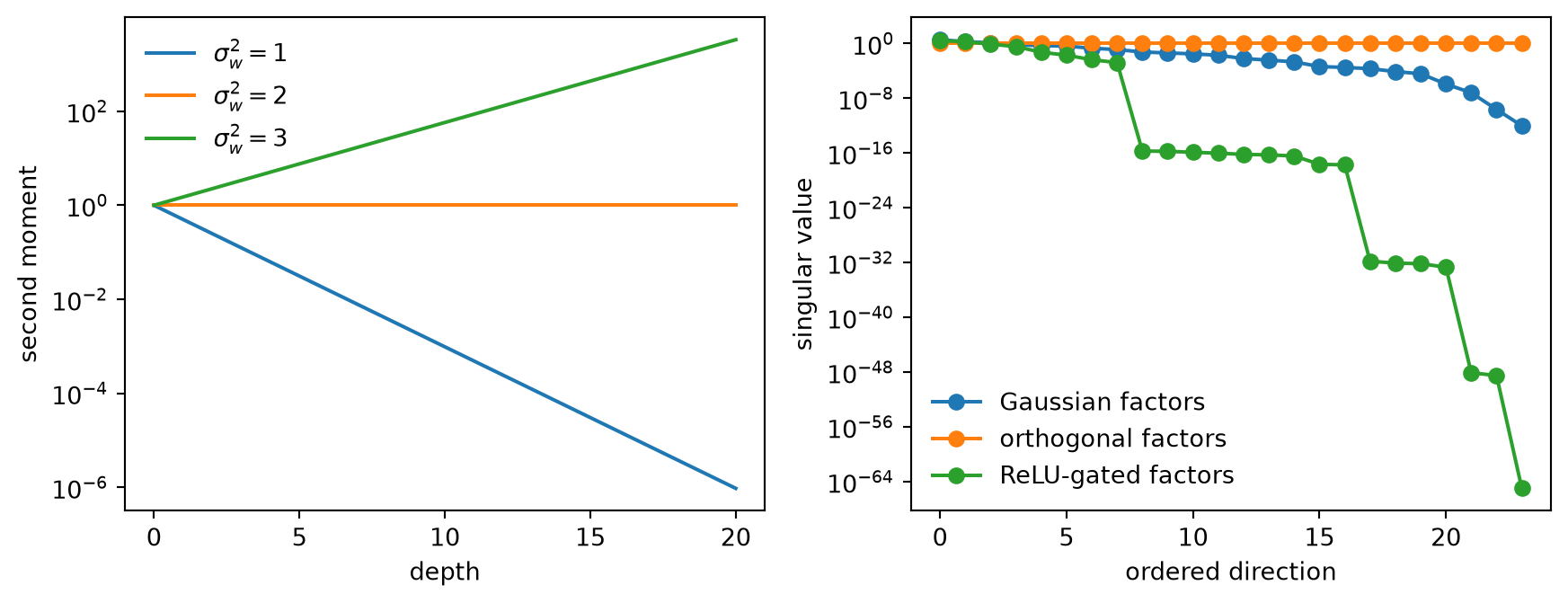
The theorem identifies a boundary: scale one decays by \(2^{-\ell}\), scale two is fixed, and scale three grows by \((3/2)^\ell\). It does not say that a finite network exactly follows the recursion, nor that scale two has a well-conditioned input-output Jacobian.

14.2 The moment survived; the distinction did not

A one-input moment cannot say whether two inputs remain distinguishable. Take equal-moment inputs and write their normalized inner product as \(c_\ell\). In the same wide Gaussian model, zero-bias ReLU propagation closes on a second scalar map.

Theorem 14.2 (Wide-model two-input correlation recursion) For two equal-moment inputs under the assumptions of Theorem 14.1,

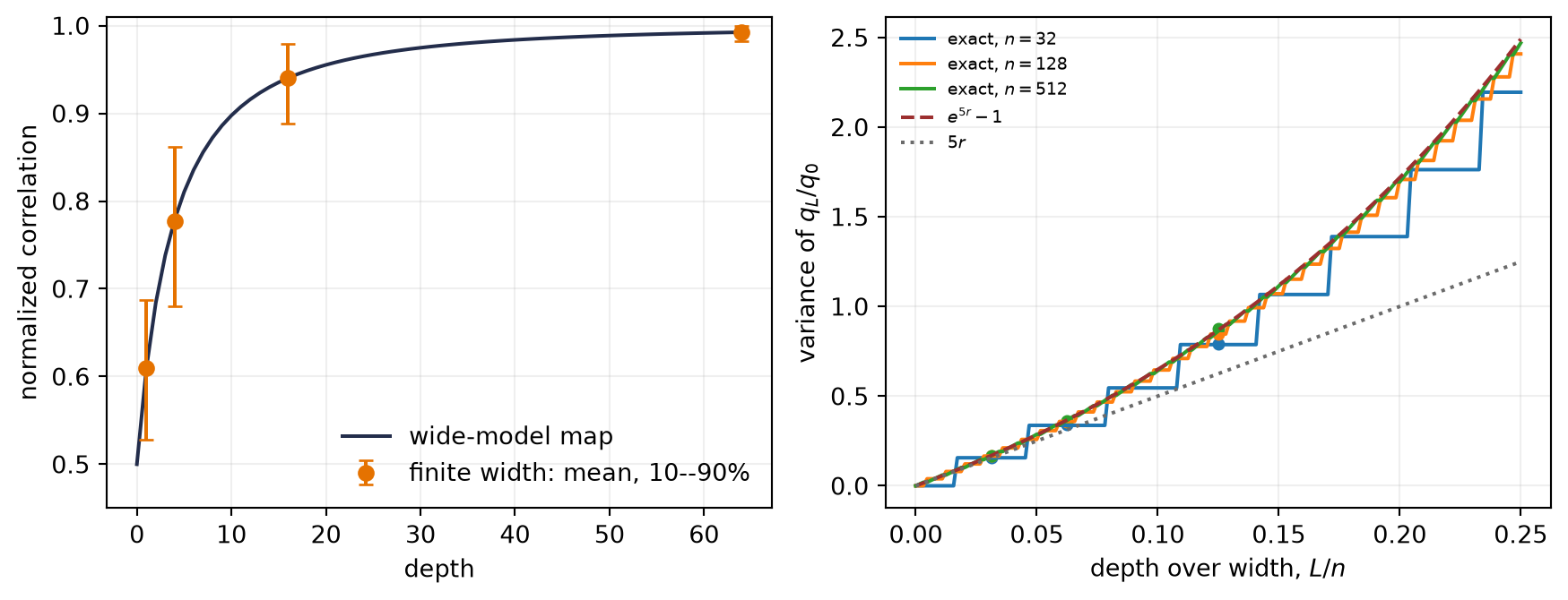
\[ c_{\ell+1}=\frac{\sqrt{1-c_\ell^2} +(\pi-\arccos c_\ell)c_\ell}{\pi}. \tag{14.3}\]

For zero bias, ReLU homogeneity cancels the weight scale from this normalized map. At the variance-critical scale \(\sigma_w^2=2\), each input’s moment stays fixed while every finite initial angle tends toward alignment. If \(c_\ell=\cos\psi_\ell\) and \(\psi_\ell\) is small, then \(\psi_{\ell+1}=\psi_\ell-\psi_\ell^2/(3\pi)+O(\psi_\ell^3)\), so \(\psi_\ell\asymp 1/\ell\).

Diagnostic derivation

The two preactivations are correlated Gaussians. Integrating the product of their positive parts over the angle between them gives Equation 14.3. Expanding \(\sin\psi-\psi\cos\psi=\psi^3/3+O(\psi^5)\) near alignment gives the stated angle recurrence. Thus local pair separation is marginal, yet finite-angle separation still decays polynomially rather than remaining fixed.

The closed form in Equation 14.3 is the degree-one arc-cosine kernel introduced by Cho and Saul (2009); Williams (1997) is the Gaussian-process covariance antecedent. Here the standard name arrives only after the normalized correlation object and its wide-model assumptions are fixed.

This is the missing contract behind the scalar critical point. The structure kept every norm and slowly lost the difference between its inputs. Changing only \(\sigma_w^2\) changes the magnitude traces but not this normalized ReLU correlation trace; three weight scales do not create three pair-geometry regimes.

The forward and backward gains should also be named separately. Let \(\chi_{\parallel}\) be the derivative of the one-input moment map at its fixed point, and let \(\chi_{\perp}\) be the infinitesimal pair-separation gain. The second factor also appears in the mean-square backward recursion. They coincide for the scale-invariant piecewise-linear family used here, but that coincidence is a property of the family, not a general law connecting forward criticality to gradient preservation.

14.3 Width is relative to depth

The wide map now needs its own trust instrument. In the finite-width critical ReLU model, let \(q_\ell=n^{-1}\sum_i(h_i^{(\ell)})^2\). Conditional on the previous layer,

\[ \frac{q_{\ell+1}}{q_\ell}=R_\ell =\frac{2}{n}\sum_{i=1}^n (Z_i)_+^2, \qquad Z_i\overset{\mathrm{iid}}{\sim}\mathcal N(0,1). \tag{14.4}\]

Theorem 14.3 (Exact finite-width moment-fluctuation control) With independent Gaussian weights of variance \(2/n\) across layers, zero bias, and ReLU coordinates,

\[ \E\!\left[\frac{q_L}{q_0}\right]=1, \qquad \var\!\left(\frac{q_L}{q_0}\right) =\left(1+\frac5n\right)^L-1. \tag{14.5}\]

Therefore the variance is \(5L/n+O((L/n)^2)\) only while \(L/n\) is small. If \(L,n\to\infty\) together with \(L/n\to r\), the same control approaches \(e^{5r}-1\), not a line.

Proof

For \(Y=(Z)_+^2\), symmetry gives \(\E Y=1/2\) and \(\E Y^2=\E[Z^4\mathbf 1_{Z>0}]=3/2\), hence \(\var(Y)=5/4\). Thus \(\E R_\ell=1\) and \(\var(R_\ell)=5/n\). Independent layer weights make the multipliers independent, so \(\E[(q_L/q_0)^2]=(1+5/n)^L\). Subtracting the squared mean proves the result.

Evaluate the wide two-input correlation control.
Load its seeded finite-width check.
Evaluate the exact depth-to-width fluctuation control.
Load the seeded moment-ratio checks.
Plot both contracts and test the declared perturbative boundary.

from book_support.criticality_figure import plot_pair_width_controls
from trainable_harness import (
    relu_correlation_trace,
    relu_moment_fluctuation_variance,
)

# [1]
pair_trace = relu_correlation_trace(0.5, 64)
# [2]
pair_claim = verify_claim("c14-pair-geometry-001", expected_harness=pin)
pair_final_mean = pair_claim["result"]["finite_width_correlation"]["64"]["mean"]
# [3]
exact_at_check = relu_moment_fluctuation_variance(512, 64)
# [4]
width_claim = verify_claim("c14-depth-width-001", expected_harness=pin)
points = width_claim["result"]["points"]
max_relative_deviation = max(
    abs(row["sample_variance"] / row["exact_variance"] - 1)
    for row in points
)
# [5]
assert abs(pair_final_mean - pair_trace[-1]) < 2e-3
assert exact_at_check > 5 * (64 / 512)
assert max_relative_deviation < 0.025
fig = plot_pair_width_controls(
    pair_trace, pair_claim, width_claim,
    relu_moment_fluctuation_variance,
)
print("pair correlation at depth 64: " f"{pair_trace[-1]:.6f}")
print("largest Monte Carlo relative deviation: " f"{max_relative_deviation:.3%}")

pair correlation at depth 64: 0.992491
largest Monte Carlo relative deviation: 1.756%

Two panels. Normalized correlation begins at one half and rises toward one through depth, with finite-width mean points and 10-to-90-percent bars near the wide-limit curve. Moment-ratio variance rises against depth divided by width; exact finite-width curves and Monte Carlo points bend above the straight small-r tangent and approach an exponential double-limit curve. — Figure 14.1: Left: at critical ReLU scale, each input keeps its moment while two inputs align; finite-width means follow the wide correlation map. Right: the exact moment-fluctuation variance bends away from its 5L/n tangent as depth over width grows. The Monte Carlo points check the finite-width identity rather than replacing it.

Claims c14-pair-geometry-001, c14-depth-width-001 · seeds: SHA-256-derived 3972769481 and 3834729383 · dtype: FP64 · device: CPU · estimators: 2,048-trial pair-correlation summaries and 200,000-trial population variances · pair artifact · depth/width artifact

The final wide-model correlation is \(0.992491\); the finite-width mean differs by about \(2\times10^{-6}\). Across the nine fluctuation checks, the largest Monte Carlo deviation from the exact variance is under \(1.8\%\). The seeded points validate the implementation. The exact curve carries the claim.

Field note: an approximation names its small parameter

Every usable limit in this book buys solvability with a declared small quantity: a step–curvature product, a noise-to-signal ratio, a covering radius, and now a depth-to-width ratio. The claim, retained order, and order of limits travel together; the claim dies where that contract stops being small. The first audit question for a clean approximation is therefore: which quantity did it assume was small, and how large is that quantity in the run on your screen?

14.4 Average control does not survive multiplication

The scalar recursion is easiest to trust after carrying it twice. Set \(q_0=1\), zero bias, and \(\sigma_w^2=2(1+\varepsilon)\). For rectified coordinates,

\[ q_1=1+\varepsilon,\qquad q_2=(1+\varepsilon)^2,\qquad q_L=(1+\varepsilon)^L. \tag{14.6}\]

At \(\varepsilon=0\), the average second moment is fixed at every depth. For a small nonzero mismatch, depth compounds the local error: the relevant quantity is \(L\log(1+\varepsilon)\), not \(\varepsilon\) alone.

Now compare the directional statement. The two matrices

\[ \matr J_1=\operatorname{diag}(\sqrt2,0),\qquad \matr J_2=\operatorname{diag}(0,\sqrt2) \]

each have mean squared singular value one, yet \(\matr J_2\matr J_1=\matr 0\). Two layers can therefore be mean-square critical individually while their derivative product destroys every direction. Repeating the scalar recursion to depth \(L\) controls an average under its independence model; controlling the product requires directional or spectral information at the same depth.

Load the chapter-pinned signal-propagation instruments.
Plot the ReLU moment recursion at three scales.
Recreate the registered Gaussian and orthogonal matrix products.
Insert ReLU gates from one finite-width forward pass at critical scale.
Compare all three spectra and verify both committed claims.

import matplotlib.pyplot as plt
import numpy as np
from hashlib import sha256

# [1]
from trainable_harness import deep_linear_product, relu_variance_trace

# [2]
fig, axes = plt.subplots(1, 2, figsize=(9.2, 3.6))
for scale in (1.0, 2.0, 3.0):
    axes[0].semilogy(relu_variance_trace(1.0, scale, 20), label=fr"$\sigma_w^2={scale:g}$")
axes[0].set(xlabel="depth", ylabel="second moment")
axes[0].legend(frameon=False)
# [3]
rng = np.random.default_rng(6214); n = 24; depth = 12
gaussian = [
    rng.normal(size=(n, n)) / np.sqrt(n) for _ in range(depth)
]
orthogonal = [
    np.linalg.qr(rng.normal(size=(n, n)))[0] for _ in range(depth)
]
# [4]
sg = np.linalg.svd(deep_linear_product(gaussian), compute_uv=False)
so = np.linalg.svd(deep_linear_product(orthogonal), compute_uv=False)
gated_seed = int(sha256(b"c14-gated-product").hexdigest()[:8], 16)
gated_rng = np.random.default_rng(gated_seed)
gated_state = gated_rng.normal(size=n)
gated_factors, active_counts = [], []
for _ in range(depth):
    weights = gated_rng.normal(size=(n, n)) * np.sqrt(2 / n)
    preactivation = weights @ gated_state
    gate = (preactivation > 0).astype(float)
    active_counts.append(int(gate.sum()))
    gated_factors.append(gate[:, None] * weights)
    gated_state = np.maximum(preactivation, 0)
sgated = np.linalg.svd(
    deep_linear_product(gated_factors), compute_uv=False
)
axes[1].semilogy(sg, "o-", label="Gaussian factors")
axes[1].semilogy(so, "o-", label="orthogonal factors")
axes[1].semilogy(sgated, "o-", label="ReLU-gated factors")
axes[1].set(xlabel="ordered direction", ylabel="singular value")
axes[1].legend(frameon=False)
fig.tight_layout()
# [5]
claim = verify_claim("c14-criticality-001", expected_harness=legacy_pin)
gated_claim = verify_claim("c14-gated-product-001", expected_harness=legacy_pin)
assert np.isclose(
    sg[0],
    claim["result"]["gaussian_product"]["maximum"],
    atol=1e-12,
)
assert active_counts == gated_claim["result"]["active_coordinates_by_layer"]
assert int(np.sum(sgated > 1e-10)) == gated_claim["result"][
    "jacobian_rank_tolerance_1e-10"
]
print("claim c14-criticality-001: verified")
print("claim c14-gated-product-001: verified")

claim c14-criticality-001: verified
claim c14-gated-product-001: verified

Two panels. The first shows activation second moment decaying for scale 1, constant for scale 2, and growing for scale 3. The second shows ordered singular values: an orthogonal product is flat at one, a Gaussian linear product spreads, and a ReLU-gated product at critical variance has only eight singular values above one times ten to the minus ten. — Figure 14.2: Left: a scalar critical point separates decay from growth. Right: average preservation does not imply directional preservation; the orthogonal linear control stays isometric, while Gaussian products spread and a finite ReLU-gated product also loses rank.

Claims c14-criticality-001, c14-gated-product-001 · seed: 6214 · dtype: FP64 · device: CPU · estimator: finite-product singular spectrum · artifact

The gated product is not an independent random-matrix toy. Its diagonal gates come from one forward pass through the same finite-width compositional structure whose Jacobian is being measured. At the variance-critical scale \(2/n\), the twelve layers retain between 8 and 20 active coordinates each, but the final Jacobian has only eight singular values above \(10^{-10}\). Its largest singular value is about \(2.63\) and its smallest is numerically zero. This one realization does not define a law for nonlinear Jacobians; it shows exactly where the deep-linear isometry control stops being the network itself.

14.5 Trace control is not edge control

For an input-output Jacobian \(\matr J\in\mathbb R^{m\times n}\),

\[ \frac1n\operatorname{tr}(\matr J^{\mathsf T}\matr J) =\frac1n\sum_i\sigma_i(\matr J)^2. \tag{14.7}\]

Theorem 14.4 (Mean-square preservation does not imply isometry) The quantity in Equation 14.7 is the mean squared stretch over an orthonormal input basis. It can equal one while the smallest singular value is zero and the largest is \(\sqrt n\).

Proof

The trace identity follows from the SVD. The diagonal matrix \(\operatorname{diag}(\sqrt n,0,\ldots,0)\) has mean squared singular value one and the stated edges.

Dynamical isometry asks for substantially more: the singular values of the relevant Jacobian should cluster near one (Pennington et al. 2017). Orthogonal factors solve the deep-linear control exactly. Nonlinear gates, finite width, correlations, biases, normalization, and trained weights change the product; orthogonality at initialization is an instrument, not a universal cure.

The word critical is therefore incomplete until it names a rung:

Contract	Observable	What it can certify	What it cannot exclude
one-input magnitude	\(q_\ell\)	average scale survives	two inputs become indistinguishable
pair geometry	\(c_\ell\) or \(\psi_\ell\)	separation contracts, expands, or is marginal	derivative directions are ill-conditioned
derivative geometry	singular values of \(\matr J\)	directional stretch and rank	the infinite-width model is inaccurate
approximation trust	\(L/n\) with retained order	the declared expansion is controlled	training leaves the declared scaling regime

The first three rows diagnose the compositional structure. The fourth audits the theory used to describe it. In particular, an infinite-width calculation can make training linearized by suppressing feature movement under its declared parameterization and time horizon. The feature-learning branch is mapped in Beyond This Volume; no width-only diagnosis is licensed here (Jacot et al. 2018; Lee et al. 2019; Chizat et al. 2019; Roberts and Yaida 2022).

14.6 The de-branded object first

We have derived variance-preserving initialization from a moment recursion. The Rosetta appendix carries the conventional aliases for search and ties each to its fan-in/fan-out and nonlinearity assumptions. The mathematics decides which moment a name actually covers.

Named wrong answer: every activation has one critical initialization

The moment map may produce a scale-invariant critical curve, a tuned point at a zero fixed point, a half-stable boundary, or no usable critical point in the declared family. Even when a scalar critical point exists, it controls one average statistic, not finite-width fluctuations, pair geometry, spectral edges, or numerical range.

14.7 Check yourself

At zero bias with ReLU and weight scale \(2(1+\varepsilon)\), what is the moment after \(L\) layers? At the exact scalar critical point, why can two inputs still align? For \(L/n=1/8\), which is the claim: \(5L/n\), the exact finite-width formula, or its simultaneous-limit curve? Finally, what do the mean squared singular value and lower spectral edge say for \(\operatorname{diag}(\sqrt2,0)\), and which statement governs a gradient component aligned with the second coordinate?

14.8 Okay, so —

Inherited: C11’s reverse product and C08’s two spectral edges now describe signal propagation.
Changed: “critical” is separated into magnitude, pair, derivative, and approximation-trust contracts.
Instrumented: four claims compare moment recursion, pair correlation, depth-to-width fluctuations, and complete product spectra.
Established: preserving a scalar moment neither preserves finite-angle distinctions nor controls Jacobian edges; \(L/n\) marks where the wide approximation accumulates finite-width corrections.
Unresolved: Which invariances and null directions does a coordinate-wise normalization choose when it resets scale?

14.9 Sources and further reading

The Gaussian covariance antecedent is Williams (1997), and the ReLU closed form is the degree-one arc-cosine kernel of Cho and Saul (2009). Two-input signal propagation follows Poole et al. (2016) and Schoenholz et al. (2017); dynamical-isometry diagnostics follow Pennington et al. (2017). Orthogonal initialization as a controlled dynamical system appears in Saxe et al. (2014). Variance-preserving initialization was developed for saturating and rectified compositional structures by Glorot and Bengio (2010) and He et al. (2015). For a derivational companion to the moment and pair-correlation recursions, and for a systematic leading finite-width expansion whose trust parameter is depth over width, see Roberts and Yaida (2022); begin with Chapter 5, Sections 5.1, 5.4, and 5.5.

Reading order. Begin with Cho and Saul (2009) for the closed form, continue with Schoenholz et al. (2017) for the one- and two-input maps and Pennington et al. (2017) for the Jacobian spectrum, then use Roberts and Yaida (2022) to audit the depth-to-width expansion and order of limits.

14.10 Exercises

(Pencil.) Derive Equation 14.2 for an odd saturating nonlinearity and identify its small-variance linearization. Decide whether the fixed point is stable from one side, both sides, or neither. Route: Core. Estimated time: 25 minutes. Prerequisite: C04 fixed points. Deliverable: derivation plus stability classification. Hint: differentiate the moment map at the fixed point.
(Code.) Repeat the product experiment across 100 seeds. Plot distributions of trace, lower edge, and upper edge separately. Route: Core. Estimated time: 45 minutes. Prerequisite: C08 spectrum summaries. Deliverable: three matched-seed distributions and a one-paragraph verdict. Hint: do not average the lower and upper edges together.
(Pencil.) For \(\matr J=\matr D_L\matr W_L\cdots\matr D_1\matr W_1\), show that \(\operatorname{rank}(\matr J)\) cannot exceed the smallest gate rank. Explain why this bound can be loose. Route: Core. Estimated time: 20 minutes. Prerequisite: rank inequalities. Deliverable: proof and one strict example. Hint: apply the rank inequality one factor at a time.
(Audit.) Build the implication graph among moment preservation, infinitesimal pair preservation, finite-angle preservation, mean-square Jacobian preservation, dynamical isometry, and trainability. Break every invalid arrow with a counterexample or a missing assumption. In particular, locate the invalid transfer from \(\chi_\perp=1\) to finite-angle preservation and state the needed smoothness or uniformity condition. Route: Extension. Estimated time: 50 minutes. Prerequisite: this chapter. Deliverable: annotated implication graph. Hint: Equation 14.3 is marginal locally but not constant at finite angle.
(Code.) Reproduce Figure 14.1 for a smooth saturating activation. Estimate \(\chi_\parallel\) and \(\chi_\perp\) separately, and classify the critical point without assuming they coincide. Route: Extension. Estimated time: 75 minutes. Prerequisite: Gaussian quadrature or Monte Carlo. Deliverable: two gain estimates, a pair trace, and a boundary statement. Hint: perturb the diagonal and off-diagonal kernel coordinates independently.
(Audit.) Paper audit: Locate a paper that uses “critical” and complete the Mathematical object, Resolution of the theory, Dynamic regime, Assumption stress test, Discriminating control, and Transfer verdict fields of the Paper Autopsy Protocol. Name its small parameter, retained order, and order of limits. As an agent-generated-proof control, remove one independence or width assumption silently, identify the first invalid step, and state the weakest repair. Route: Research. Estimated time: 90 minutes. Prerequisite: C11–C14. Deliverable: six-field autopsy plus repaired statement. Hint: “infinite width” is not an order of limits until depth is named.