13 The Mean Gradient Is Not the Regime: Conditional Noise and Stochastic Dynamics

SG · Sub-Gaussian safe zone · LG · Landscape and update geometry Geometric supporting · Dynamic primary · Algorithmic supporting

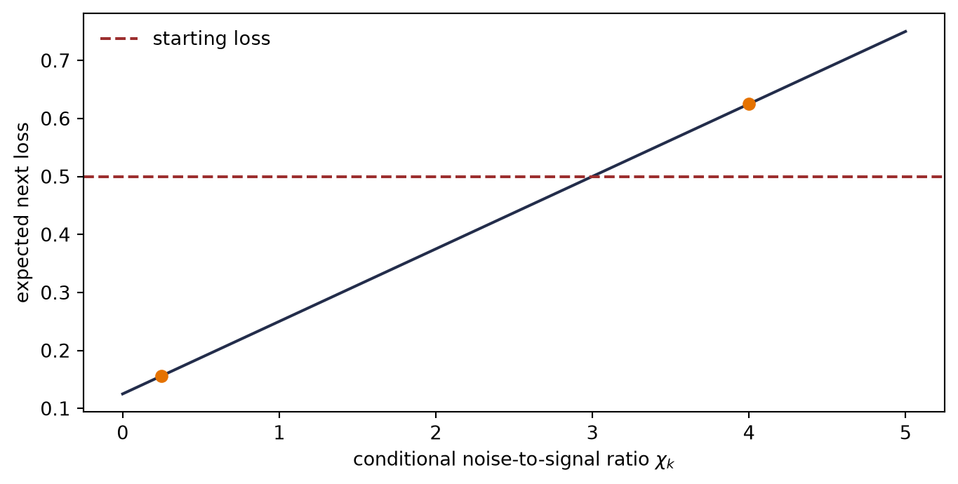
At \(w=1\), the scalar loss \(f(w)=w^2/2\) has gradient one. Take the update \(w^+=w-0.5g\), where \(g=1+\xi\) is conditionally unbiased. If \(\E[\xi^2]=0.25\), then \(\E[f(w^+)]=0.15625\): expected descent from the initial loss \(0.5\). If \(\E[\xi^2]=4\), then \(\E[f(w^+)]=0.625\): expected ascent. The current state, mean gradient, curvature, and step size are identical. Only the conditional dispersion changed.

Prediction

An optimizer plot reports a mean gradient norm but not the estimator’s conditional variance or tail behavior. Can it identify whether step decay or batch growth is the relevant intervention? Name one observation that would make those two interventions distinguishable.

13.1 Declare the estimator before its variance

Let \(\mathcal F_k\) contain everything known before sampling at step \(k\). A usable stochastic-gradient contract is

\[ \E[\vect g_k\mid\mathcal F_k]=\nabla f(\vect w_k),\qquad \E[\|\vect g_k-\nabla f(\vect w_k)\|^2\mid\mathcal F_k] \leq \sigma_k^2. \tag{13.1}\]

The conditioning matters. Sampling without replacement, correlated examples, adaptive data selection, clipping, and quantization can all alter the mean or dispersion. “Gradient noise” without a filtration, averaging rule, and target is not yet a mathematical object.

Theorem 13.1 (Conditional expected descent) Suppose \(f\) is \(L\)-smooth and Equation 13.1 holds with finite conditional second moment. For \(\vect w_{k+1}=\vect w_k-\alpha\vect g_k\),

\[ \E[f(\vect w_{k+1})\mid\mathcal F_k] \leq f(\vect w_k)-\alpha\left(1-\frac{L\alpha}{2}\right) \|\nabla f(\vect w_k)\|^2+\frac{L\alpha^2}{2}\sigma_k^2. \tag{13.2}\]

Proof

Apply the smoothness upper bound to \(-\alpha\vect g_k\), condition on \(\mathcal F_k\), and use \(\E\|\vect g_k\|^2=\|\nabla f(\vect w_k)\|^2+ \E\|\vect g_k-\nabla f(\vect w_k)\|^2\).

When the variance bound is tight, the right side predicts descent whenever

\[ \alpha < \frac{2/L}{1+\sigma_k^2/\|\nabla f(\vect w_k)\|^2}. \tag{13.3}\]

The ratio \(\chi_k=\sigma_k^2/\|\nabla f(\vect w_k)\|^2\) is the diagnostic axis. Small \(\chi_k\) is gradient-dominated; large \(\chi_k\) is noise-dominated. This is an internal regime ledger, not a fifth narrative sigil.

Load the chapter-pinned stochastic-regime instruments.
Evaluate the exact scalar quadratic expectation over a variance grid.
Mark the two opening estimators.
Compute the conditional safe-step threshold.
Verify the committed claim before interpreting the curve.

import matplotlib.pyplot as plt
import numpy as np

# [1]
from trainable_harness import (
    centered_pareto_clip_bias,
    conditional_safe_step,
    scalar_quadratic_regime,
)

# [2]
ratios = np.linspace(0.0, 5.0, 200)
expected = [
    scalar_quadratic_regime(1.0, 0.5, ratio).expected_next_loss
    for ratio in ratios
]
# [3]
fig, axis = plt.subplots(figsize=(7.2, 3.7))
axis.plot(ratios, expected, color="#232D4B")
axis.axhline(
    0.5, color="#9C2F2F", linestyle="--", label="starting loss"
)
axis.scatter(
    [0.25, 4.0], [0.15625, 0.625], color="#E57200", zorder=3
)
axis.set(
    xlabel=r"conditional noise-to-signal ratio $\chi_k$",
    ylabel="expected next loss",
)
axis.legend(frameon=False)
fig.tight_layout()
# [4]
assert np.isclose(conditional_safe_step(1.0, 4.0, 1.0), 0.4)
# [5]
claim = verify_claim("c13-regime-001", expected_harness=pin)
assert claim["result"]["high_noise"]["expected_next_loss"] == 0.625
print("claim c13-regime-001: verified")

claim c13-regime-001: verified

Line chart of expected next loss against noise-to-signal ratio. It rises from 0.125 and crosses the initial loss 0.5; marked points at ratios 0.25 and 4 have expected losses 0.15625 and 0.625. — Figure 13.1: The same mean gradient crosses from expected descent to expected ascent as conditional noise grows. The dashed line is the starting loss, not a fitted threshold.

Claim c13-regime-001 · seed: none (exact expectation) · dtype: FP64 · device: CPU · estimator: conditional second moment · artifact

13.2 Watch the regime change while the objective stays fixed

The opening calculation compares two estimators at one state. A training run changes the denominator of \(\chi_k\): even if the noise scale stays constant, the gradient norm can shrink. To see that transition, keep the objective \(f(w)=w^2/2\), nominal step \(0.12\), per-example noise standard deviation \(0.8\), and batch size \(16\) fixed for 80 steps. At each step, estimate the variance of the batch mean from the 16 per-example gradients and divide by the exact full-gradient norm squared.

The same executable control then asks three adjacent questions. Does batch averaging follow the promised \(1/b\) law? Does momentum help the exact ill-conditioned quadratic while amplifying stochastic forcing? What remains of a variance-only diagnosis when the noise has no finite second moment?

Derive independent seeds from the claim identities.
Run one online quadratic and estimate its conditional ratio each step.
Verify batch-mean variance across four batch sizes.
Compare plain and momentum recurrences with and without shared noise.
Reuse C06’s exact clipping bias for an infinite-variance Pareto model.
Plot the controls and verify the committed claim.

# [1]
def derived_seed(label):
    return int(sha256(label.encode()).hexdigest()[:8], 16)

# [2]
online_rng = np.random.default_rng(derived_seed("c13-online-regime"))
state, online_step, noise_sd, batch_size = 1.0, 0.12, 0.8, 16
online_losses, online_chi = [], []
for _ in range(80):
    gradients = state + online_rng.normal(scale=noise_sd, size=batch_size)
    online_losses.append(0.5 * state**2)
    online_chi.append(
        gradients.var(ddof=1) / batch_size / max(state**2, 1e-30)
    )
    state -= online_step * gradients.mean()
first_crossing = int(np.flatnonzero(np.asarray(online_chi) >= 1)[0])

# [3]
batch_sizes, trial_count = np.array([1, 4, 16, 64]), 20_000
batch_streams = np.random.SeedSequence(
    derived_seed("c13-batch-scaling")
).spawn(len(batch_sizes))
observed_batch_variances = []
for size, stream in zip(batch_sizes, batch_streams, strict=True):
    means = np.random.default_rng(stream).normal(
        scale=noise_sd, size=(trial_count, int(size))
    ).mean(axis=1)
    observed_batch_variances.append(means.var(ddof=1))
observed_batch_variances = np.asarray(observed_batch_variances)
theory_batch_variances = noise_sd**2 / batch_sizes

# [4]
curvatures = np.array([0.01, 1.0])
momentum_step, beta = 0.5, 0.9
def deterministic_trace(memory):
    point, velocity, trace = np.ones(2), np.zeros(2), []
    for _ in range(80):
        trace.append(0.5 * np.sum(curvatures * point**2))
        velocity = memory * velocity + curvatures * point
        point -= momentum_step * velocity
    return np.asarray(trace)

plain_trace = deterministic_trace(0.0)
momentum_trace = deterministic_trace(beta)
forcing_rng = np.random.default_rng(derived_seed("c13-momentum-noise"))
plain = np.ones((20_000, 2))
momentum = plain.copy()
velocity = np.zeros_like(momentum)
for _ in range(500):
    forcing = forcing_rng.normal(scale=0.2, size=plain.shape)
    plain -= momentum_step * (curvatures * plain + forcing)
    velocity = beta * velocity + curvatures * momentum + forcing
    momentum -= momentum_step * velocity
stochastic_losses = np.array([
    np.mean(0.5 * np.sum(curvatures * plain**2, axis=1)),
    np.mean(0.5 * np.sum(curvatures * momentum**2, axis=1)),
])

# [5]
pareto_bias = centered_pareto_clip_bias(1.5, [2.0, 4.0, 16.0, 64.0])

# [6]
fig, axes = plt.subplots(2, 2, figsize=(9.2, 6.2))
axes[0, 0].semilogy(online_chi, color="#232D4B")
axes[0, 0].axhline(1, color="#9C2F2F", linestyle="--")
axes[0, 0].set(xlabel="step", ylabel=r"estimated $\chi_k$")
axes[0, 1].loglog(
    batch_sizes, observed_batch_variances, "o-", color="#232D4B",
    label="observed",
)
axes[0, 1].loglog(
    batch_sizes, theory_batch_variances, "--", color="#9C2F2F",
    label=r"$\sigma^2/b$",
)
axes[0, 1].set(xlabel="batch size", ylabel="variance of batch mean")
axes[0, 1].legend(frameon=False)
axes[1, 0].semilogy(plain_trace, color="#9C2F2F", label="plain")
axes[1, 0].semilogy(momentum_trace, color="#232D4B", label="momentum")
axes[1, 0].set(xlabel="deterministic step", ylabel="quadratic loss")
axes[1, 0].legend(frameon=False)
axes[1, 1].bar(
    ["plain", "momentum"], stochastic_losses,
    color=["#9C2F2F", "#232D4B"],
)
axes[1, 1].set(ylabel="mean loss after 500 noisy steps")
for axis in axes.flat:
    axis.grid(alpha=0.2)
fig.tight_layout()

controls_claim = verify_claim("c13-regime-controls-001", expected_harness=pin)
assert first_crossing == controls_claim["result"]["online_crossing"][
    "first_chi_at_least_one"
]
assert np.allclose(
    observed_batch_variances,
    [
        controls_claim["result"]["batch_scaling"]["by_batch_size"][str(size)][
            "observed_variance"
        ]
        for size in batch_sizes
    ],
)
print(f"first chi crossing: step {first_crossing}")
print(
    "noisy loss, plain/momentum: "
    f"{stochastic_losses[0]:.4f}/{stochastic_losses[1]:.4f}"
)
print("Pareto clip bias, C=2/4/16/64: " + "/".join(
    f"{value:.3f}" for value in pareto_bias.values()
))

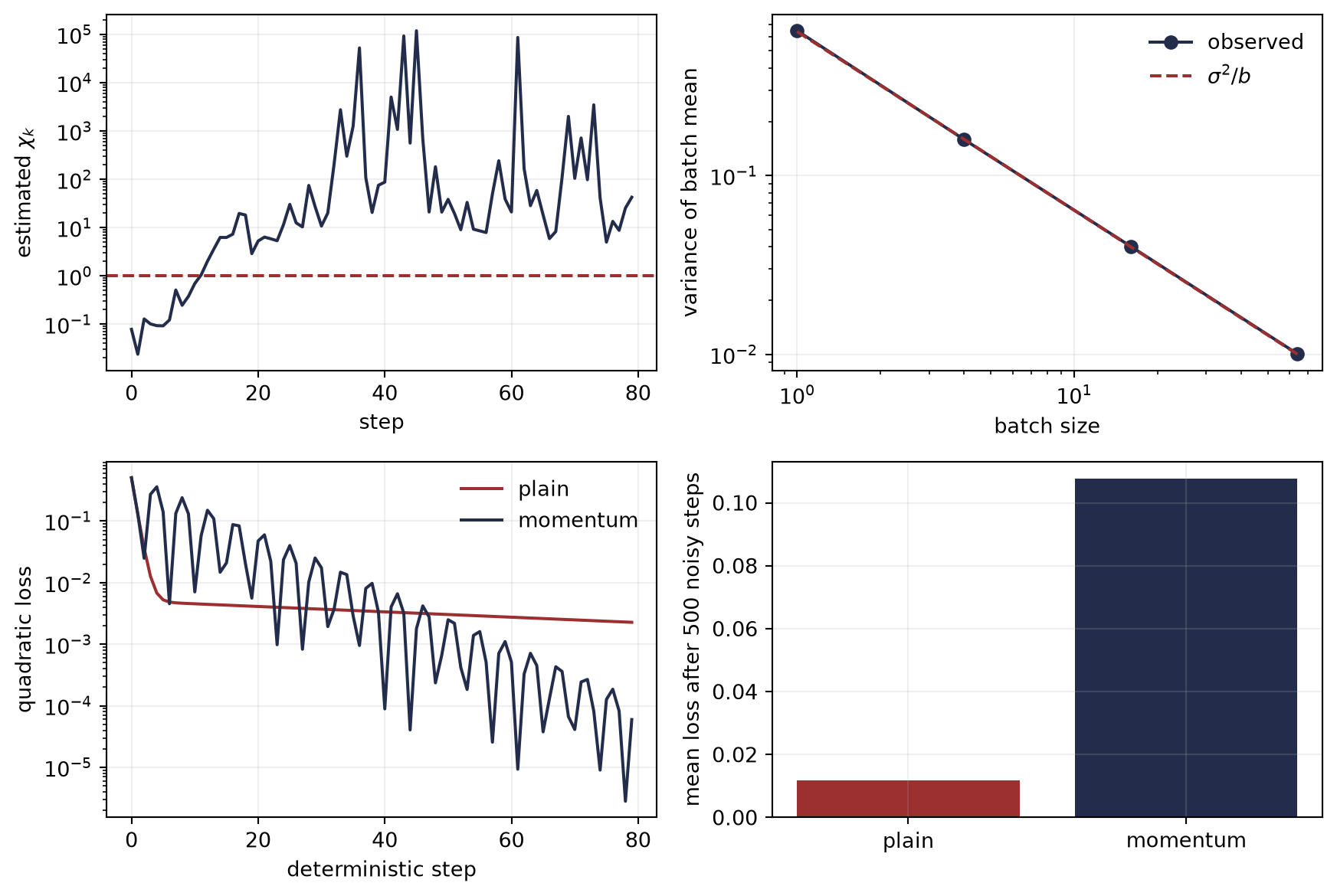
first chi crossing: step 11
noisy loss, plain/momentum: 0.0117/0.1077
Pareto clip bias, C=2/4/16/64: -0.894/-0.756/-0.459/-0.244

Four panels. The online noise-to-signal ratio crosses one near step 11. Observed batch-mean variance follows a one-over-b line. Momentum lowers deterministic quadratic loss faster than plain descent. With additive noise, the same momentum produces a much higher terminal mean loss. — Figure 13.2: Four controls separate four mechanisms. The online run crosses chi equals one with objective, step, noise scale, and batch fixed; independent batch means follow the one-over-b variance law; momentum improves the deterministic ill-conditioned control but amplifies shared stochastic forcing. The Pareto clipping calculation is reported separately because its variance is infinite.

The measured ratio first exceeds one at step 11. This is a transition in the diagnostic regime, not a change in the objective or nominal schedule. The batch panel follows \(\sigma^2/b\) because the code deliberately uses independent, identically distributed finite-variance samples. It is a control for that assumption, not evidence that real training batches obey it.

For the two-mode quadratic with curvatures \(0.01\) and \(1\), momentum uses

\[ r^2-(1+\beta-\alpha\lambda)r+\beta=0. \tag{13.4}\]

When \(0\le\beta<1\), this exact scalar control is stable for \(0<\alpha\lambda<2(1+\beta)\). With \(\alpha=0.5\) and \(\beta=0.9\), the deterministic loss after 80 steps is about \(1.20\times10^{-4}\), versus \(2.24\times10^{-3}\) without memory. Under shared additive forcing, however, the mean losses after 500 steps are about \(0.108\) and \(0.0117\). Memory changed the noise filter as well as the deterministic roots.

Finally, the centered Pareto model with shape \(3/2\) has a finite mean and infinite variance. Its \(\chi_k\) is undefined, so no larger batch can be justified by a \(\sigma^2/b\) calculation. C06’s exact clipping audit still applies: thresholds \(2,4,16,64\) induce mean biases about \(-0.894,-0.756,-0.459,-0.244\). Clipping makes the update bounded while changing its target, and the bias disappears only as the threshold recedes.

13.3 Batch size is an assumption-bearing lever

For a mean of \(b\) conditionally independent, identically distributed per-example estimators with finite variance, the variance becomes \(\sigma_k^2/b\). Then Equation 13.3 explains the linear-scaling heuristic only in the noise-dominated range: multiplying batch and step by the same factor approximately preserves the variance penalty while that factor is small enough that the smoothness term remains benign. Correlation, changing data distributions, or infinite variance break the derivation.

The inequality also explains why “decrease the step” and “increase the batch” can address the same term while having different compute and communication costs. C01’s traffic contract must therefore accompany the statistical one.

13.4 Clipping repairs a tail by changing the target

Let \(g=-9\) with probability \(0.1\) and \(g=19/9\) otherwise. Its mean is one and variance is \(100/9\). Clipping to \([-2,2]\) lowers variance to \(1.44\) but moves the mean to \(1.6\). The estimator is no longer unbiased for the original gradient. This is the C06 lesson inside an update: variance reduction and target preservation are separate audit columns.

Named wrong answer: clipping makes the theorem apply

Clipping supplies bounded tails for the clipped estimator. It does not make that estimator unbiased for the unclipped gradient. A convergence argument must carry the bias term or redefine the objective it targets.

13.5 Acceleration is a branch, not a survey

The paired witness supplies the promised boundary: the exact quadratic recurrence can improve the deterministic slow mode while the same \(\beta\) amplifies stochastic forcing. Chebyshev schedules, conjugate-gradient polynomials, and other acceleration variants remain branches. The trunk question is which resolution the theory uses—global, local, direction-aware, or finite-horizon—and which regime the evidence probes.

13.6 Check yourself

With \(L=1\), gradient norm two, and conditional variance 12, what is the noise-to-signal ratio and the threshold in Equation 13.3? If four independent copies are averaged, what changes? Which two steps of that answer fail for the shape-\(3/2\) Pareto model?

13.7 Okay, so —

Inherited: C04’s curvature modes and C06’s tail boundary remain the controls.
Changed: an update claim now begins with a conditional estimator, not the word “stochastic.”
Instrumented: an exact one-step claim and an online control separate regime crossing, batch scaling, momentum filtering, and clipping bias.
Established: expected descent depends on both smoothness and a noise-to-signal ratio.
Unresolved: Why can preserving one scalar variance through depth still destroy individual derivative directions?

13.8 Sources and further reading

The conditional descent calculation is standard in large-scale stochastic optimization; see Bottou et al. (2018) and the foundational approximation scheme of Robbins and Monro (1951). The heavy-ball control originates with Polyak (1964). The named diagonal-moment method and its decoupled-decay variant are Kingma and Ba (2015) and Loshchilov and Hutter (2019); this chapter uses them as literature bridges, not as a substitute for the estimator contract. Heavy-tailed gradient evidence is discussed by Simsekli et al. (2019). The 2026 ICML tutorial by Mark Schmidt supplied the intellectual map from theory resolution to regime diagnosis; the equations and qualifications here are derived on the page rather than attributed to the tutorial.

Reading order. Start with Bottou et al. (2018) for conditional descent and batch effects, use Polyak (1964) for the exact momentum control and Simsekli et al. (2019) to stress the finite-variance assumption, then read Schmidt (2026) last as a map of research resolutions and regimes.

13.9 Exercises

(Pencil.) Derive the exact stationary variance of scalar quadratic descent with additive zero-mean noise and compare it with Equation 13.2.
(Pencil.) Apply the Jury criterion to Equation 13.4 and derive \(0<\alpha\lambda<2(1+\beta)\) for \(0\le\beta<1\). State why this is an exact-quadratic result rather than a global nonlinear guarantee.
(Code.) Replace the two-point noise by both a finite-variance heavy tail and the shape-\(3/2\) Pareto model. Across seeds and batch sizes, compare mean, median, clipped estimate, and failure of the sample-variance diagnostic.
(Code.) Reproduce the online crossing with shared random streams while varying only batch size. Report first-crossing time, estimator variance, and total examples processed; do not rank batches by step count alone.
(Audit.) Paper audit: For an optimizer paper, complete the Mathematical object, Dynamic regime, Estimator and comparison contract, Assumption stress test, Discriminating control, and Transfer verdict fields of the Paper Autopsy Protocol. Name the conditional estimator and decide whether clipping changes its target.
(Audit.) A warmup–stable–decay schedule is explained as three successive regimes. Identify the observable needed to label each transition, then give one rival explanation based on changing curvature and one based on changing estimator noise.