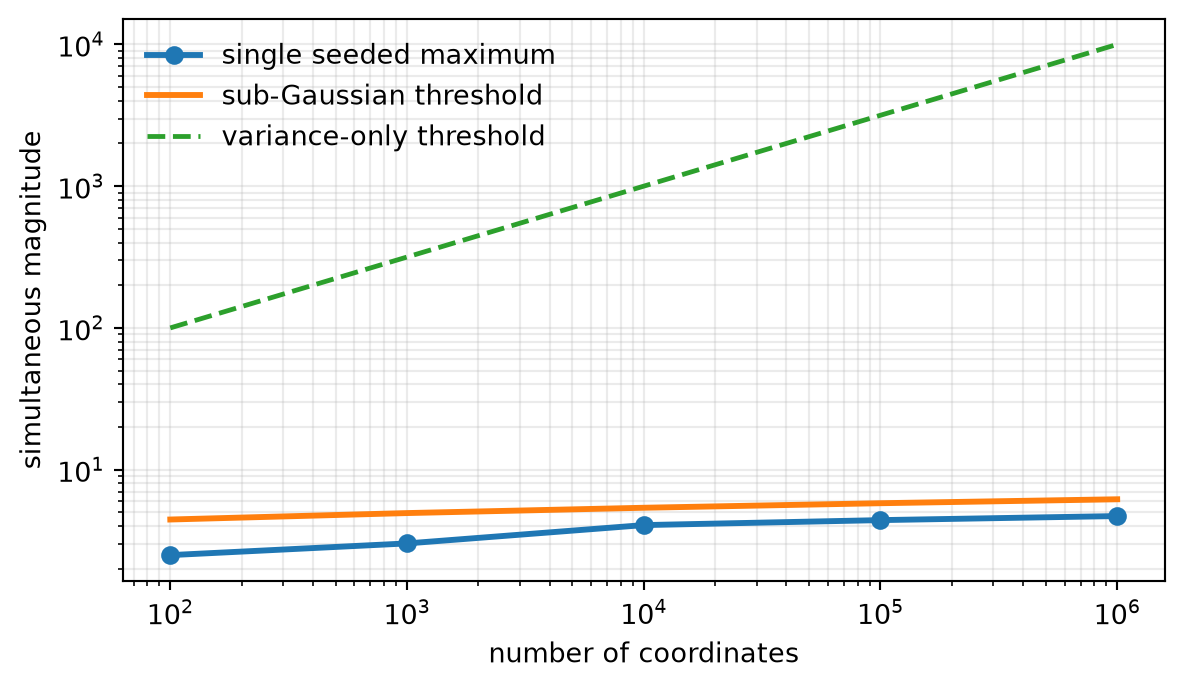
Draw one standard-normal vector of length \(100\), then one of length one million. In the seeded witness below, their largest magnitudes are \(2.50\) and \(4.71\).
The number of opportunities grew by ten thousand. The maximum did not.
ImportantPrediction
If the number of coordinates grows by a factor of ten, should a 99%-simultaneous deviation threshold:
grow by a factor of ten;
grow by a factor of \(\sqrt{10}\); or
increase only through a logarithm?
Choose one, then name the tail assumption your answer needs.
5.1 A million chances to fail
The study uses one independent random stream per vector length. Each maximum is a single seeded witness, not an estimate of the expected maximum. The comparison curve is a theorem-derived threshold at failure probability \(\delta=0.01\).
Load the chapter-pinned concentration instruments.
Draw one independent standard-normal vector at each declared size.
Compute the simultaneous sub-Gaussian threshold.
Assert the witness remains inside the threshold.
Plot observed maxima against logarithmic and polynomial scales.
Figure 5.1: Observed coordinate maxima grow slowly across vector sizes from 100 to one million. The sub-Gaussian 99%-simultaneous threshold grows as the square root of a logarithm, while a variance-only union-bound threshold grows as the square root of the count. The observed line is one seeded witness; it does not estimate the expected maximum or certify an unknown distribution’s tail class.
The bound pays for one million opportunities through \(\sqrt{\log(10^6)}\), not \(\sqrt{10^6}\). The final printed number, \(7.2141\), is a model calculation for one billion independent standard-normal coordinates under the same proxy scale. The code did not generate a billion values.
The geometric problem is now precise: we need a tail envelope strong enough to survive a union over many quantities, and we need a scale that composes under weighted sums.
5.2 Exponentiate, then optimize
For a centered real random variable \(X\), suppose
\[
\E\!\left[e^{\lambda X}\right]
\le
\exp\!\left(\frac{\sigma^2\lambda^2}{2}\right)
\qquad
\text{for every }\lambda\in\mathbb{R}.
\tag{5.1}\]
We call \(\sigma\) a sub-Gaussian MGF proxy scale. It is an admissible envelope, not automatically the smallest such scale and not automatically the standard deviation.
Theorem 5.1 (MGF envelope implies a Gaussian tail) Under Equation 5.1, for every \(t\ge0\),
The exponent is a quadratic in \(\lambda\), minimized at \(\lambda^\star=t/\sigma^2\). Substitution gives \(\Pr(X\ge t)\le e^{-t^2/(2\sigma^2)}\). Apply the same argument to \(-X\) and add the two tail probabilities. \(\square\)
This is the exponential lift: a probability question becomes a one-dimensional optimization problem. The theorem does not manufacture an MGF bound. It tells us what the bound buys once we establish it.
For a Rademacher sign \(\varepsilon\in\{-1,+1\}\) with equal probabilities,
Thus a random sign has proxy scale one. The inequality can be proved by comparing the power series or by checking that \(e^{-\lambda^2/2}\cosh(\lambda)\) decreases for \(\lambda>0\).
Theorem 5.2 (Independent weighted sums) Let \(X_1,\ldots,X_d\) be independent, centered random variables with MGF proxy scales \(\sigma_1,\ldots,\sigma_d\). For fixed coefficients \(\vect{a}\in\mathbb{R}^d\),
Independence is doing identifiable work: it turns one MGF into a product. Without it, Equation 5.4 is not licensed.
If the \(X_j\) are Rademacher and \(a_j=1/\sqrt{d}\), then \(\sum_j a_j^2=1\). The sum keeps proxy scale one at every width. Width alone does not cause the scalar projection to explode; coefficient energy decides.
5.4 Pay only a logarithm for simultaneous control
Theorem 5.3 (Simultaneous sub-Gaussian control) Suppose \(X_1,\ldots,X_m\) each satisfy Equation 5.2 with the same proxy scale \(\sigma\). Mutual independence is not required. For any \(0<\delta<1\), with probability at least \(1-\delta\),
Set the last expression equal to \(\delta\) and solve for \(t\). \(\square\)
Dependence can make the union bound loose, but it does not invalidate the guarantee. Independence was essential for closing weighted sums; it is not essential for union-bounding already available marginal tails.
WarningNamed wrong answer: ‘A billion variables require a billion-sigma threshold’
The number of opportunities appears inside a logarithm under a sub-Gaussian tail envelope. The threshold at \(m=10^9\) and \(\delta=0.01\) is about \(7.21\sigma\), not \(10^9\sigma\). Change the tail class, however, and the scaling can change with it.
Theorem 5.4 (Gaussian input, nonlinear diagnostic) Let \(\vect{G}\sim\mathcal{N}(\vect{0},\matr{I}_d)\) and let \(f:\mathbb{R}^d\to\mathbb{R}\) be \(L\)-Lipschitz in Euclidean distance, with \(L>0\). There are universal constants \(c,C>0\) such that
Proof with pointer. This is Gaussian concentration, stated in the Orlicz form of Vershynin’s second-edition Theorem 5.2.3 (Vershynin 2026). The tail form follows from the \(\psi_2\) characterization below. The useful extension is not a new exponent but a new object: \(f\) can be nonlinear. For example, \(f(\vect{x})=\norm{\matr{A}\vect{x}}_2\) is \(\norm{\matr{A}}_{\mathrm{op}}\)-Lipschitz, so its fluctuation around its mean inherits a sub-Gaussian scale.
The theorem controls fluctuation around a declared center; it does not compute that center. Its standard-Gaussian input is also part of the contract. The statement is not a dependence theorem for arbitrary inputs and does not extend unchanged to heavy-tailed data.
5.5 Four instruments for the same safe zone
Sometimes the MGF is easy to calculate. Sometimes moments or a tail bound are what the problem exposes. The following theorem makes those entry points interchangeable at the level of tail class, not at the level of identical constants.
Theorem 5.5 (Equivalent sub-Gaussian diagnostics) For a centered real random variable \(X\), the following properties are equivalent up to universal constant factors:
\(\Pr(|X|\ge t)\le2e^{-t^2/K_1^2}\) for all \(t\ge0\);
\((\E|X|^p)^{1/p}\le K_2\sqrt{p}\) for every \(p\ge1\);
\(\E e^{X^2/K_3^2}\le2\);
\(\E e^{\lambda X}\le e^{K_4^2\lambda^2}\) for every real \(\lambda\).
The best admissible constants \(K_1,\ldots,K_4\) are comparable up to universal factors.
The full equivalence is proved in Vershynin’s second-edition Proposition 2.6.1 (Vershynin 2026). One direction is immediate here: property 3 and Markov’s inequality give
It is a population quantity. An empirical moment curve may reveal a violation or suggest a regime, but a finite sample cannot certify what happens beyond its largest observation.
Available object
Diagnostic question
Boundary
tail probabilities
does \(-\log\Pr(|X|\ge t)\) grow quadratically?
rare tails may be unseen
moments
does \(\norm{X}_p/\sqrt p\) remain bounded?
high-order estimates are unstable
exponential-square moment
is a candidate \(K\) integrable?
sample averages can hide divergence
MGF
is log-MGF bounded by a quadratic for all \(\lambda\)?
local-in-\(\lambda\) control gives local tails
NoteField note: proxy variance is not variance
Differentiating an exact MGF at zero connects its second derivative to variance, so every valid proxy variance is at least the actual variance. Equality is special. Record “MGF proxy scale” when that is the object used by the proof.
5.6 Width without scale explosion
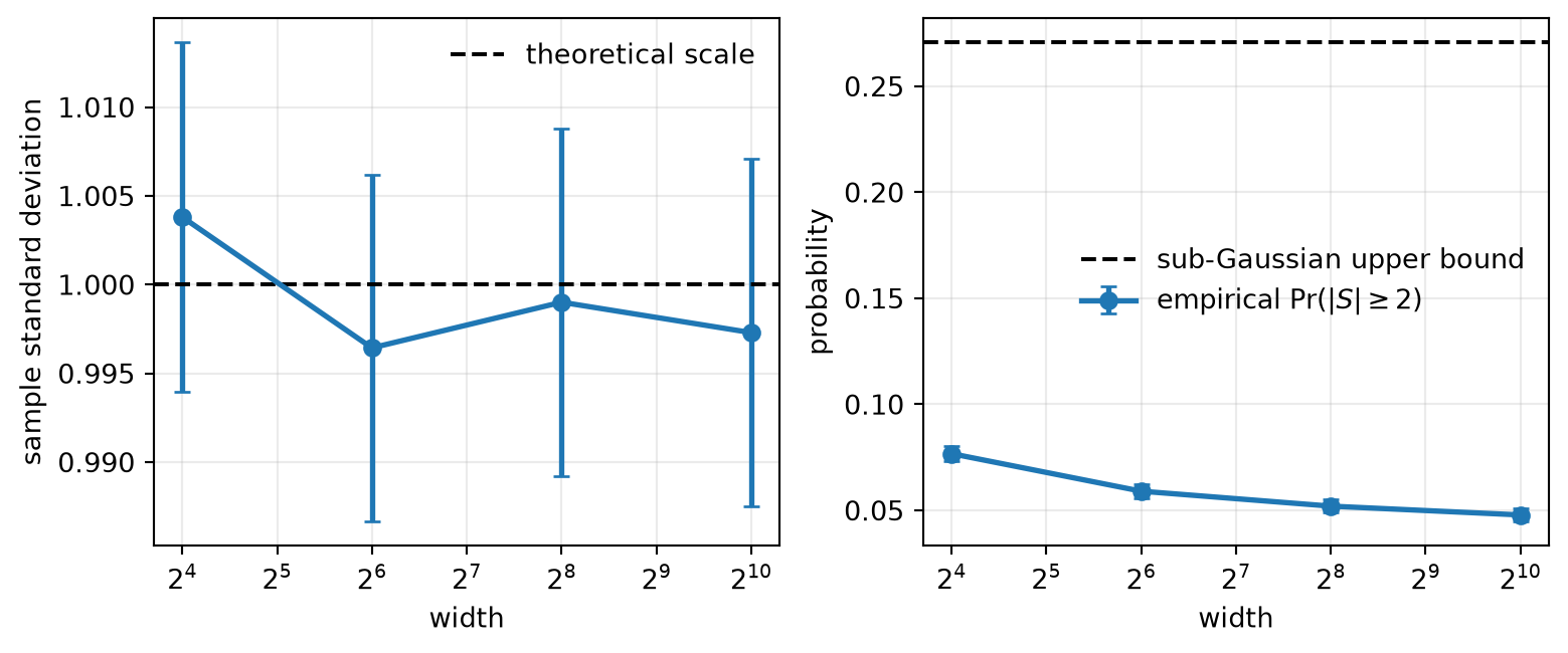
The next study uses independent Rademacher signs and the normalized coefficients \(a_j=1/\sqrt d\). For each width, 20,000 independent projections estimate the mean, sample standard deviation, and the two-sided event \(|S|\ge2\). Each width receives a separate named seed.
Declare widths, trial count, coefficient norm, and seed policy.
Generate normalized Rademacher projections.
Estimate mean, standard deviation, and a two-sided tail probability.
Report estimator uncertainty and assert order-one scale.
Figure 5.2: Normalized Rademacher projections retain sample standard deviation near one from width 16 through 1024, as predicted by coefficient energy. The empirical event probability for absolute projection at least two varies with the finite lattice and approaches the Gaussian-like regime; the loose sub-Gaussian upper bound is shown only as a guarantee.
The sample standard deviations range from about \(0.996\) to \(1.004\). That is evidence for this seeded protocol, with approximate standard error about \(0.005\) for each standard deviation. The theorem explains why the scale should remain order one: \(\norm{\vect{a}}_2=1\) at every width.
The tail bound \(2e^{-2}\approx0.271\) is deliberately loose. It is a valid envelope, not a prediction of the exact tail probability.
5.7 Geometry meets the finite grid
Suppose a computation produces \(m\) centered scalar quantities with proxy scale \(\sigma\). Equation Equation 5.5 gives a high-probability envelope for their maximum. C03 then asks whether that envelope fits the declared storage range and whether the sums forming each quantity use an adequate accumulator.
For \(m=10^9\), \(\delta=0.01\), and \(\sigma=1\), the model threshold \(7.21\) is far below FP16’s largest finite value. That statement alone does not guarantee safe training:
the proxy scale may drift;
coordinates may cease to be sub-Gaussian;
depth can multiply scales;
intermediate reductions can overflow even when outputs do not;
an implementation can change the accumulation contract.
The safe zone is a diagnostic hypothesis with a numerical consequence, not a branding phrase. C14 will derive when initialization keeps the coefficient energy controlled across depth. C06 has the nearer obligation: it will square a sub-Gaussian quantity and show why the same tail model no longer applies.
TipCheck yourself
Let \(m=10^7\), \(\delta=10^{-3}\), and proxy scale \(\sigma=0.5\). Compute the simultaneous threshold from Equation 5.5. If all variables are identical copies of the same random variable rather than independent, does the theorem remain valid? Which earlier proof step changes?
5.8 Okay, so —
Inherited: C03 supplied the range/accumulation contract, and C04 showed why controlling one direction is not enough when many modes coexist.
Changed: Randomness is now described by a tail class and proxy scale that can survive simultaneous control.
Instrumented: The harness computes simultaneous thresholds, seeded maxima, weighted-sign projections, empirical tails, and moment-growth profiles.
Established: A quadratic MGF envelope yields Gaussian tail decay, independent weighted sums add proxy variances, a union bound charges only \(\sqrt{\log m}\), and Lipschitz diagnostics of a standard Gaussian input concentrate around their own means.
Unresolved: Which tail class replaces global sub-Gaussian control after a square or product changes the moment-generating function?
5.9 Sources and further reading
Chernoff’s exponential method supplies the optimization view of tail bounds (Chernoff 1952). Hoeffding develops probability inequalities for sums of bounded independent variables (Hoeffding 1963). Vershynin gives the modern sub-Gaussian equivalence, Orlicz norm, and Gaussian Lipschitz concentration used here (Vershynin 2026).
For the general theory, use Vershynin (2026); this chapter’s contribution is the precision-facing safe-zone diagnostic and its explicit failure boundary.
Reading order. Start with Vershynin (2026) for the reusable equivalences, then read Chernoff (1952) and Hoeffding (1963) for the original exponential-method and bounded-sum viewpoints.
5.10 Exercises
(Pencil.) Optimize the exponent. Repeat the proof of Theorem 5.1 when the MGF bound is known only for \(|\lambda|\le\lambda_0\). Derive the range of \(t\) in which the quadratic optimizer remains admissible and state what happens outside it.
(Pencil.) Dependence audit. Give two examples with identical sub-Gaussian marginals: one with independent coordinates and one with all coordinates equal. Compare their exact maxima and the common union-bound guarantee. Explain why validity and sharpness are separate questions.
(Code.) Maxima as an estimator. Replace the single opening witness with repeated maxima at each feasible count. Predeclare trial counts, report the empirical median and a quantile interval, and keep the total draw budget fixed across design choices.
(Code.) Coefficient geometry. Compare three coefficient sequences: uniform \(1/\sqrt d\), one-spike, and geometrically decaying, all normalized to the same \(\ell_2\) norm. Measure tails and explain what the MGF theorem predicts identically and what the exact distributions retain.
(Audit.) The empirical certificate. A report computes \(\norm{X}_p/\sqrt p\) for \(p\le8\) on 10,000 observations and declares the population sub-Gaussian. Predict a contamination distribution that is likely to evade the sample, then state a defensible empirical conclusion.
(Audit.) Paper audit: Hoeffding’s bounded-sum inequality. Complete the Mathematical object, Evidence culture and interface, Assumption stress test, and Transfer verdict fields for the primary paper and extract the independence assumption, the bounded-range quantity, and the tail exponent for a weighted sum. Map each object to the MGF proxy language of this chapter and identify any constant or scope that cannot be transferred verbatim.
Chernoff, Herman. 1952. “A Measure of Asymptotic Efficiency for Tests of a Hypothesis Based on the Sum of Observations.”The Annals of Mathematical Statistics 23 (4): 493–507. https://doi.org/10.1214/aoms/1177729330.
Hoeffding, Wassily. 1963. “Probability Inequalities for Sums of Bounded Random Variables.”Journal of the American Statistical Association 58 (301): 13–30. https://doi.org/10.1080/01621459.1963.10500830.
Vershynin, Roman. 2026. High-Dimensional Probability: An Introduction with Applications in Data Science. 2nd ed. Cambridge Series in Statistical and Probabilistic Mathematics. Cambridge University Press. https://www.math.uci.edu/~rvershyn/papers/HDP-book/HDP-book.html.