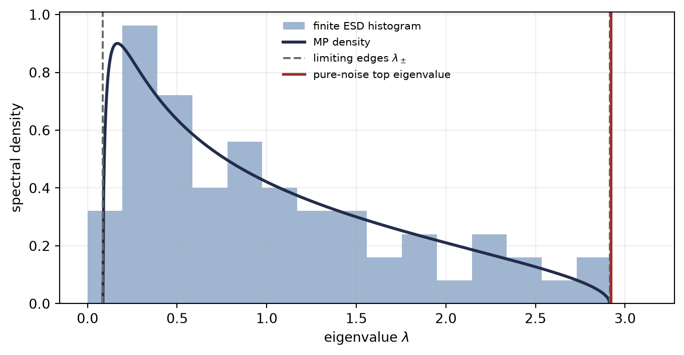
Generate \(128\) observations with \(64\) independent standard-normal coordinates. The population covariance is exactly \(\matr{I}_{64}\). For the seeded realization below, the largest eigenvalue of the sample covariance is
The Marchenko–Pastur upper edge at aspect ratio \(\gamma=64/128=1/2\) is
\[
\lambda_+=(1+\sqrt{\gamma})^2\approx2.914.
\]
The sample crosses the edge even though there is no population signal to find.
ImportantPrediction
Does \(\lambda_{\max}>\lambda_+\) reject the pure-noise model? If not, what must be calibrated before the word “signal” is justified?
9.1 The outlier is made of noise
The matrix convention matters. Let \(\matr{X}\in\mathbb{R}^{m\times n}\) have observations in rows and coordinates in columns. Here the population mean is known to be zero, so the estimator is the sample second moment
Its eigenvalues are the squared singular values of \(\matr{X}/\sqrt m\). C08 located those edges; this chapter instruments the mass between them. To prevent a hidden seed search, the witness seed is the first 32 bits of the SHA-256 digest of the registered phenomenon ID c09-bulk-not-verdict.
Load the chapter-pinned spectral instruments.
Generate the predeclared pure-noise witness.
Form the known-zero-mean second-moment estimator and compute its exact eigenvalues.
Evaluate the Marchenko–Pastur density under the matching aspect ratio.
Plot the finite empirical spectrum and mark the limiting support edges.
Figure 9.1: A pure-noise finite spectrum can cross an asymptotic edge. The histogram is the exact eigenvalue spectrum of one seeded 64-coordinate sample covariance from 128 independent standard-normal observations. The curve is the Marchenko–Pastur limiting density for the matching aspect ratio. The top eigenvalue lies beyond the limiting upper edge; that crossing is the symptom, not yet a rejection rule.
harness=ch-09 wheel=0d4b6e953774
mean eigenvalue=1.021187; lambda_max=2.921244
MP edges=[0.085786, 2.914214]
The overlay is visually persuasive and logically insufficient. The Marchenko–Pastur curve is a limit under a declared generative model. The histogram is one finite random measure. Neither object says how often the largest finite eigenvalue crosses the limiting support.
9.2 Name the estimator before naming the law
Three similar-looking matrices answer different questions:
Mean contract
Computation
Denominator meaning
population mean known to be zero
\(\frac1m\sum_i\vect{x}_i\vect{x}_i^{\mathsf T}\)
unbiased second moment under the declared mean
population mean unknown; maximum-likelihood Gaussian convention
Changing centering or denominator changes the finite null. The opening uses the first row of the table. A report that says only “we computed the covariance” has not specified its estimator.
For a symmetric matrix \(\matr{M}\) with eigenvalues \(\lambda_1,\ldots,\lambda_n\), define its empirical spectral distribution
This is not merely a histogram. It is the exact probability measure that places mass \(1/n\) at each finite eigenvalue. A histogram adds a binning choice for visualization.
Theorem 9.1 (Trace moments of an empirical spectrum) For every nonnegative integer \(k\),
Integrating against the point masses in Equation 9.2 gives the same sum divided by \(n\). For \(k=0\), the identity says that the ESD has total mass one. \(\square\)
The first moment is normalized trace. For the sample covariance,
The largest eigenvalue is a different functional. A correct mean does not pin the upper edge, just as C08’s Frobenius average did not pin both singular edges.
9.3 The bulk law is asymptotic
Theorem 9.2 (Marchenko–Pastur law) Let \(\matr{X}\in\mathbb{R}^{m\times n}\) have independent entries with mean zero, variance one, and finite fourth moment. Suppose \(m,n\to\infty\) with
Then the ESD of \(\widehat{\matr{\Sigma}}=\matr{X}^{\mathsf T}\matr{X}/m\) converges almost surely, weakly, to the Marchenko–Pastur measure. Its continuous density is
Independence and proportional growth produce a deterministic fixed-point equation for the limiting transform, whose inversion yields Equation 9.4. Establishing almost-sure convergence and controlling the resolvent error is the technical work. We use the theorem diagnostically and point to the original paper for the full argument (Marchenko and Pastur 1967).
The scaling is part of the theorem. The entries of \(\matr{X}\) have variance one and the Gram matrix is divided by \(m\). Equivalently, \(\matr{A}=\matr{X}/\sqrt m\) has entry variance \(1/m\) and \(\widehat{\matr{\Sigma}}=\matr{A}^{\mathsf T}\matr{A}\). Mixing variance \(1/n\) with the edges in Equation 9.5 changes the mean spectral scale by a factor of \(m/n\).
C08’s scaled Gaussian singular edges were \(1\pm\sqrt{\gamma}\). The eigenvalue edges here are their squares. The Marchenko–Pastur law adds the missing mass between them.
WarningNamed wrong answer: ‘Above the MP edge means signal’
The support describes a limiting measure. It does not say that every eigenvalue of every finite null matrix lies inside the support. An edge crossing becomes evidence only after the finite statistic, calibration rule, false-positive budget, and alternative model are declared.
9.4 A deterministic bulk can still be a poor covariance estimate
The sample spectrum can converge to a beautiful deterministic shape while the sample covariance remains far from the population covariance in operator norm. For the isotropic case,
At fixed positive \(\gamma\), the limiting edges do not collapse to one.
Theorem 9.3 (Sub-Gaussian covariance-estimation error) Let \(\vect{X}\in\mathbb{R}^n\) be centered with covariance \(\matr{\Sigma}\), and assume that for every \(\vect{x}\),
Whiten the data: \(\vect{Z}=\matr{\Sigma}^{-1/2}\vect{X}\). The whitened rows are isotropic and sub-Gaussian, so C08 controls all singular values of their data matrix. Squaring those bounds controls \(\norm{m^{-1}\matr{Z}^{\mathsf T}\matr{Z}-\matr{I}}_{\mathrm{op}}\). Conjugating by \(\matr{\Sigma}^{1/2}\) contributes \(\norm{\matr{\Sigma}}_{\mathrm{op}}\). Vershynin gives the full expectation and high-probability bookkeeping (Vershynin 2026).
The ambient-dimension rate says that \(m\) must scale like \(n/\varepsilon^2\) for relative operator error \(\varepsilon\). C10 will replace \(n\) with an effective dimension when the population spectrum is concentrated. That promise is now contractual, not rhetorical.
9.5 Calibrate the finite statistic
Return to the opening shape. The finite null must match:
\(m=128\), \(n=64\);
independent standard-normal entries;
known population mean zero, with no sample centering;
denominator \(m\);
statistic \(\lambda_{\max}\);
false-positive rate \(\alpha=0.05\);
one predeclared look.
The next study uses \(2{,}000\) independent null matrices with a seed different from the opening witness. The 95th empirical percentile is a calibrated threshold for this contract—not a universal constant.
Reuse the declared shape and analytic Marchenko–Pastur edge.
Generate an independently seeded finite Gaussian null ensemble.
Compute the largest eigenvalue for every exact covariance matrix.
Predeclare the upper five-percent empirical threshold.
Compare the opening witness with both the asymptotic edge and finite threshold.
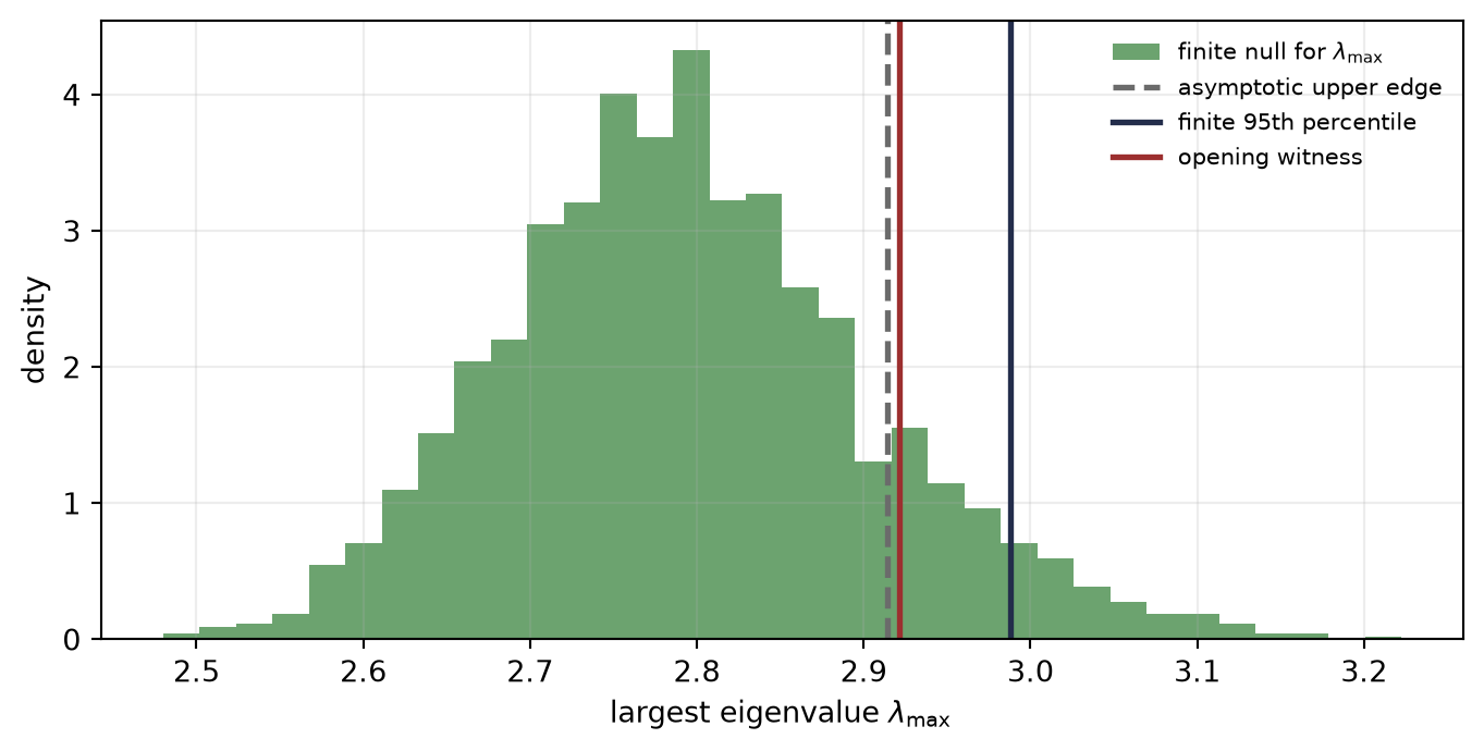
Figure 9.2: The limiting upper edge is not a finite five-percent threshold. In 2,000 independently seeded pure-noise covariance matrices of the opening shape, 13.85 percent of largest eigenvalues exceed the asymptotic edge. The opening witness crosses that edge but remains below the empirical 95th-percentile null threshold. The histogram is a distribution of one predeclared statistic, not an ESD.
null edge-crossing rate=0.1385; finite threshold=2.987940
witness=2.921244; reject at alpha=0.05: False
The result resolves the symptom. In this finite ensemble, \(13.85\%\) of pure noise matrices cross the limiting edge. The opening value \(2.921\) is above the edge but below the finite 95th percentile \(2.988\). Under this predeclared test, it is not rejected.
The threshold is only as portable as its null contract. Correlated rows, heavy-tailed coordinates, sample centering, a different aspect ratio, or a search across many layers all require recalibration.
Theorem 9.4 (Repeated-look false alarms) If each of \(K\) inspected spectra has a null event with probability at most \(\alpha\), then
\[
\Pr\{\text{at least one false alarm}\}\le K\alpha.
\]
If the looks are independent and each event has probability exactly \(\alpha\), then the probability is
\[
1-(1-\alpha)^K.
\tag{9.8}\]
Proof
The first statement is the union bound. Under independence, no false alarm occurs with probability \((1-\alpha)^K\); take the complement. \(\square\)
At twenty independent looks, a nominal five-percent per-look rule has about a \(64.2\%\) chance of at least one false alarm. If the asymptotic edge were mistaken for the threshold, the measured \(13.85\%\) per-look crossing rate would produce about a \(94.9\%\) chance of at least one crossing. Monitoring creates a multiple-comparison problem even before training dynamics enter.
NoteField note: nulls are executable specifications
Store the null generator beside the diagnostic. Record shape, orientation, centering, denominator, marginal distribution, dependence assumptions, statistic, seed, trial count, quantile method, false-positive level, and number of looks. “Compared with MP” is a picture caption; it is not a reproducible test.
9.6 Signal needs an alternative model
A finite null tells us which values are unusual under noise. It does not say which structured mechanism produced an unusual value. The smallest useful alternative is a rank-one population spike:
Even this genuine population structure need not create a separated sample eigenvalue.
Theorem 9.5 (Rank-one spiked-covariance separation) Under the model in Equation 9.9, independent standardized entries with finite fourth moment, and \(n/m\to\gamma\in(0,1)\), the largest sample eigenvalue converges almost surely to
Baik and Silverstein characterize the almost-sure limits of sample eigenvalues for finite-rank perturbations of the identity covariance (Baik and Silverstein 2006). The displayed rank-one formula is their specialization. The important diagnostic fact is the phase boundary: below \(1+\sqrt{\gamma}\), a real population spike is asymptotically absorbed at the null edge.
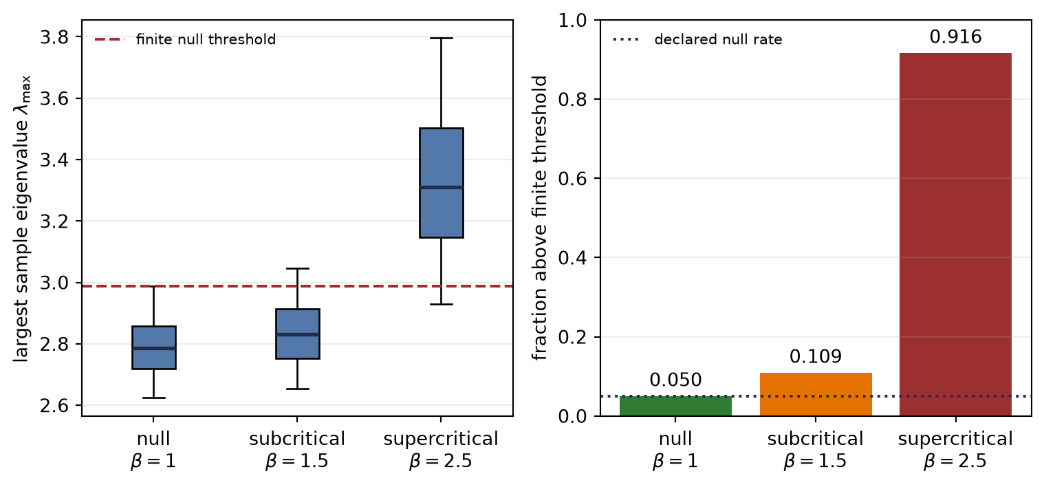
For \(\gamma=1/2\), the population threshold is about \(1.707\). The next finite study compares \(\beta=1\), a subcritical spike \(\beta=1.5\), and a supercritical spike \(\beta=2.5\), each over \(2{,}000\) independently seeded matrices. All three use the same five-percent finite null threshold from the previous study.
Declare null, subcritical, and supercritical population eigenvalues.
Generate independent finite ensembles under the rank-one Gaussian model.
Compute the exact largest sample eigenvalue in every trial.
Compare each ensemble with the previously calibrated finite null threshold.
Plot finite distributions and rejection fractions beside the asymptotic separation boundary.
Figure 9.3: A population spike is not the same as a separated sample eigenvalue. At aspect ratio one half, the subcritical population spike beta equals 1.5 remains close to the null largest-eigenvalue distribution and crosses the finite five-percent threshold in only 10.9 percent of trials. The supercritical spike beta equals 2.5 separates and crosses in 91.65 percent. Boxes span the interquartile range; whiskers show the fifth and ninety-fifth percentiles.
The subcritical model contains genuine population structure, yet most finite sample spectra do not separate from the null. Conversely, an arbitrary outlier in a learned matrix does not inherit this theorem unless the spiked covariance model is defensible.
The diagnostic hierarchy is now explicit:
Object
Question answered
Invalid shortcut
ESD
Where did this finite matrix place spectral mass?
a histogram proves the null
Marchenko–Pastur law
What bulk emerges under an iid proportional-growth null?
the limiting edge is a finite test
finite null
Is the predeclared statistic unusual at this exact shape and estimator?
unusual identifies the mechanism
spiked alternative
When does one declared population perturbation separate?
every learned outlier is a spike
A Hessian, a parameter update, and a sample covariance are all symmetric matrices after suitable products, but symmetry does not give them the same generative law. C12 will build a curvature-specific null. C14 will ask how one-layer spectra compose through depth.
TipCheck yourself
Two teams inspect the same \(50\) independently initialized layers. Team A flags every eigenvalue above the asymptotic Marchenko–Pastur edge. Team B calibrates the maximum across all \(50\) layers under a matched joint null. Which team controls the experiment-level false-positive probability? List the metadata needed to reproduce Team B’s threshold.
9.7 Okay, so —
Inherited: C08 supplied singular edges and the aspect-ratio geometry; C05 supplied a sub-Gaussian null class, and C06 warned that covariance entries are squared quantities.
Changed: two edges became a full empirical spectral measure, and the asymptotic bulk became a baseline rather than a finite verdict.
Instrumented: the harness now declares covariance orientation, centering, denominator, Marchenko–Pastur support and density, finite extreme-eigenvalue trials, and an empirical upper threshold.
Established: Marchenko–Pastur explains the limiting null mass under its assumptions; covariance estimation can still have order-one operator error; repeated looks spend a false-positive budget; and a genuine subcritical population spike can remain inside the sample bulk.
Unresolved: Which dimension should replace ambient coordinate count when most spectral mass lies in only a few directions?
9.8 Sources and further reading
Marchenko and Pastur establish the limiting empirical spectral law (Marchenko and Pastur 1967). Vershynin supplies the sub-Gaussian covariance-estimation theorem and its whitening argument (Vershynin 2026). Baik and Silverstein derive the almost-sure sample-eigenvalue limits for spiked population models (Baik and Silverstein 2006).
For the general theory, use Vershynin (2026) and the primary random-matrix papers; this chapter’s contribution is an executable finite-null calibration.
Reading order. Start with Marchenko and Pastur (1967) for the limiting bulk, use Vershynin (2026) for finite covariance error, and read Baik and Silverstein (2006) only after separating a population spike from a finite sample verdict.
9.9 Exercises
(Pencil.) Mass, mean, and edge. Construct two probability measures on four nonnegative points with the same first moment but different maxima. Realize them as ESDs of diagonal matrices. Explain why normalized trace cannot replace an upper-edge diagnostic.
(Pencil.) The zero atom. Let \(n>m\). Prove directly from rank that \(\matr{X}^{\mathsf T}\matr{X}\) has at least \(n-m\) zero eigenvalues. Show that their ESD mass tends to \(1-1/\gamma\) when \(n/m\to\gamma>1\).
(Code.) Estimator contract. Under one fixed Gaussian data generator, compare known-zero-mean division by \(m\), sample centering with division by \(m\), and sample centering with division by \(m-1\). Calibrate a separate finite largest-eigenvalue threshold for each. Report seeds, denominators, trial counts, and quantile method.
(Code.) Finite shape audit. Hold \(\gamma=1/2\) approximately fixed while increasing \(m,n\). Measure the probability that \(\lambda_{\max}\) crosses the limiting edge and the distance between the edge and the empirical 95th percentile. Do not infer a convergence rate from a log–log line without a theorem.
(Audit.) Null misspecification. Replace independent Gaussian rows with temporally correlated rows, then with heavy-tailed coordinates. Keep the old threshold long enough to measure its false-positive rate. Identify which Marchenko–Pastur and covariance-estimation assumptions were broken.
(Audit.) Paper audit: a model-specific outlier. Complete the Mathematical object, Resolution of the theory, Dynamic regime, Assumption stress test, Discriminating control, and Transfer verdict fields for Baik and Silverstein (Baik and Silverstein 2006). Extract the population model, aspect-ratio limit, moment assumptions, separation condition, almost-sure conclusion, and the quantity that remains asymptotic. Then review a spectral-outlier claim in a current machine-learning paper: state whether its matrix has the same generative model and propose a matched finite null if it does not.
Baik, Jinho, and Jack W. Silverstein. 2006. “Eigenvalues of Large Sample Covariance Matrices of Spiked Population Models.”Journal of Multivariate Analysis 97 (6): 1382–408. https://doi.org/10.1016/j.jmva.2005.08.003.
Marchenko, V. A., and L. A. Pastur. 1967. “Distribution of Eigenvalues for Some Sets of Random Matrices.”Mathematics of the USSR-Sbornik 1 (4): 457–83. https://doi.org/10.1070/SM1967v001n04ABEH001994.
Vershynin, Roman. 2026. High-Dimensional Probability: An Introduction with Applications in Data Science. 2nd ed. Cambridge Series in Statistical and Probabilistic Mathematics. Cambridge University Press. https://www.math.uci.edu/~rvershyn/papers/HDP-book/HDP-book.html.