15  Normalization Chooses an Invariance: Coordinate Statistics and Derivative Paths

NS · Numerical stability · LG · Landscape and update geometry

Geometric primary · Dynamic supporting · Algorithmic supporting

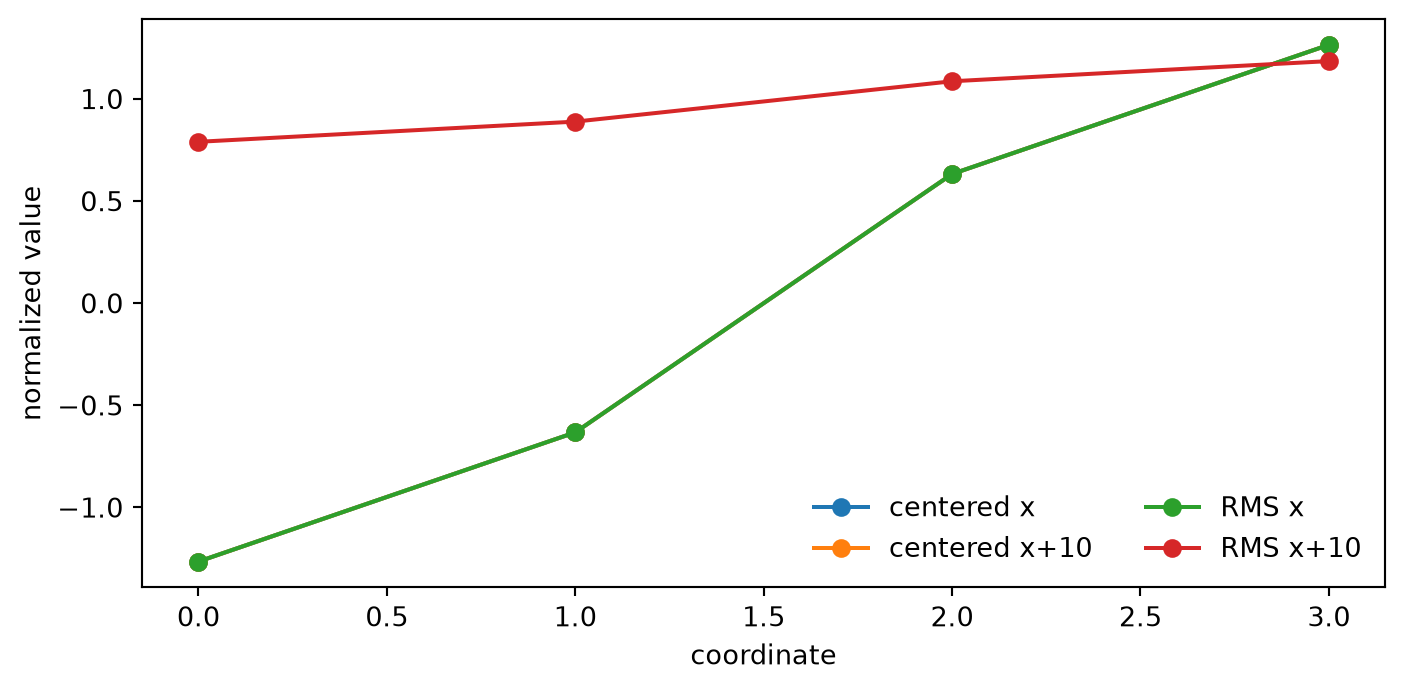
Take \(\vect x=(-2,-1,1,2)\) and shift every coordinate by ten. Centering and scaling sends both vectors to the same output. Scaling by the uncentered root mean square does not: the maximum coordinate-wise change is \(2.055\). The two maps are often offered as nearly interchangeable stabilizers, but they erase different information.

The arithmetic also matters. For FP32 values \((9998,9999,10001,10002)\), the raw-moment expression \(\operatorname{mean}(x^2)-\operatorname{mean}(x)^2\) evaluates to zero in the registered runtime, while centering first gives \(2.5\). C02’s cancellation has returned inside a standard training primitive.

ImportantPrediction

If a normalization rule is removed or replaced, what behavior should change? Answer by naming its invariance, Jacobian nullspace, statistic, placement, and precision contract—not by invoking the method name.

15.1 Two maps, two quotients

Ignoring learned affine parameters and an implementation epsilon, define

\[ \mathcal N_C(\vect x)=\sqrt d\, \frac{\matr P\vect x}{\|\matr P\vect x\|_2},\quad \matr P=\matr I-\frac1d\vect 1\vect 1^{\mathsf T}, \tag{15.1}\]

and

\[ \mathcal N_R(\vect x)=\sqrt d\,\frac{\vect x}{\|\vect x\|_2}. \tag{15.2}\]

The centered map is invariant to positive scaling and constant-coordinate translation. The RMS map is invariant to positive scaling but retains the constant component. Neither contract is universally superior; the choice is architectural information.

Theorem 15.1 (Jacobians expose the erased directions) Away from degenerate states and with zero epsilon, let \(\vect u=\vect x/\|\vect x\|\) and \(\vect v=\matr P\vect x/\|\matr P\vect x\|\). Then

\[ \matr J_R=\frac{\sqrt d}{\|\vect x\|}(\matr I-\vect u\vect u^{\mathsf T}), \qquad \matr J_C=\frac{\sqrt d}{\|\matr P\vect x\|}(\matr P-\vect v\vect v^{\mathsf T}). \tag{15.3}\]

Generically, \(\matr J_R\) has rank \(d-1\) and \(\matr J_C\) rank \(d-2\).

Proof

Differentiate \(\vect z/\|\vect z\|\) to obtain \((\matr I-\widehat{\vect z}\widehat{\vect z}^{\mathsf T})/\|\vect z\|\). For Equation 15.1, compose with the fixed projector \(\matr P\). The RMS map annihilates its radial direction. The centered map additionally annihilates \(\vect1\) because \(\matr P\vect1=0\).

1. Load the chapter-pinned normalization instruments.
2. Normalize one vector before and after a constant shift.
3. Compute both exact zero-epsilon Jacobians.
4. Compare raw-moment and centered FP32 variance.
5. Verify the registered invariance and rank claims.

import matplotlib.pyplot as plt
import numpy as np

# [1]
from trainable_harness import (
    centered_normalize,
    merge_moments,
    normalization_jacobian,
    raw_and_centered_variance,
    rms_normalize,
    stable_online_moments,
)

# [2]
x = np.array([-2.0, -1.0, 1.0, 2.0])
shifted = x + 10.0
outputs = {
    "centered x": centered_normalize(x),
    "centered x+10": centered_normalize(shifted),
    "RMS x": rms_normalize(x),
    "RMS x+10": rms_normalize(shifted),
}
fig, axis = plt.subplots(figsize=(7.4, 3.7))
for label, values in outputs.items():
    axis.plot(values, "o-", label=label)
axis.set(xlabel="coordinate", ylabel="normalized value")
axis.legend(frameon=False, ncol=2)
fig.tight_layout()
# [3]
assert np.linalg.matrix_rank(
    normalization_jacobian(x, centered=True), tol=1e-10
) == 2
assert np.linalg.matrix_rank(
    normalization_jacobian(x, centered=False), tol=1e-10
) == 3
# [4]
assert raw_and_centered_variance(
    np.array([9998, 9999, 10001, 10002])
) == (0.0, 2.5)
# [5]
claim = verify_claim("c15-invariance-001", expected_harness=pin)
assert claim["result"]["centered_shift_deviation"] == 0.0
print("claim c15-invariance-001: verified")

claim c15-invariance-001: verified

Figure 15.1: Centering and RMS-only scaling choose different equivalence classes. Centered normalization removes a constant shift; RMS normalization preserves evidence of it.

Claim c15-invariance-001 · seed: none · dtype: FP64 with paired FP32 cancellation check · device: CPU · estimator: deterministic map and Jacobian · artifact

15.2 Epsilon changes the map

Production rules use a denominator such as \(\sqrt{m_2+\varepsilon}\). Epsilon prevents division by zero and caps local amplification, but it breaks exact scale invariance when \(m_2\) is comparable to epsilon. Its value and placement are therefore part of the algorithm. Accumulating \(m_2\) in a wider format can matter even when stored activations are narrow. Raw moments should not be used when a centered statistic is intended.

Batch-coordinate normalization adds another state: running estimates used at evaluation. Those are streaming centered statistics of the kind built in C02, with the same estimator-denominator and reduction-order obligations.

15.3 Train state and evaluation state are different estimators

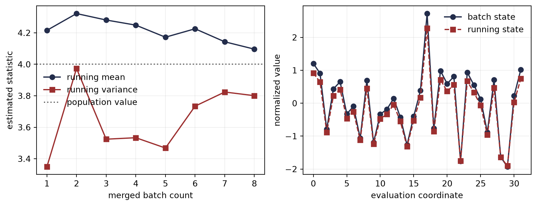
The oldest forward promise in the book now becomes executable. Draw eight training batches and one evaluation batch from the same scalar Gaussian population. There is no distribution shift. Train mode normalizes the evaluation batch using its own 32 observations; evaluation mode uses the running state merged from 256 earlier observations. The two outputs can still differ because the estimators saw different finite samples.

1. Derive a claim-specific seed and draw train and evaluation batches.
2. Build one centered state per training batch and merge the states.
3. Build the evaluation batch state with the same denominator contract.
4. Normalize the evaluation values under the two estimator states.
5. Plot convergence and output discrepancy, then verify the claim.

# [1]
running_seed = int(sha256(b"c15-running-state").hexdigest()[:8], 16)
running_rng = np.random.default_rng(running_seed)
training_batches = running_rng.normal(4, 2, size=(8, 32))
evaluation_batch = running_rng.normal(4, 2, size=32)

# [2]
batch_states = [
    stable_online_moments(batch, dtype=np.float64)
    for batch in training_batches
]
running_state = batch_states[0]
running_trace = [running_state]
for batch_state in batch_states[1:]:
    running_state = merge_moments(running_state, batch_state)
    running_trace.append(running_state)
direct_state = stable_online_moments(
    training_batches.ravel(), dtype=np.float64
)

# [3]
evaluation_state = stable_online_moments(
    evaluation_batch, dtype=np.float64
)
epsilon = 1e-5

# [4]
train_mode_output = (
    (evaluation_batch - evaluation_state.mean)
    / np.sqrt(evaluation_state.population_variance + epsilon)
)
evaluation_mode_output = (
    (evaluation_batch - running_state.mean)
    / np.sqrt(running_state.population_variance + epsilon)
)

# [5]
fig, axes = plt.subplots(1, 2, figsize=(9.2, 3.6))
batch_axis = np.arange(1, len(running_trace) + 1)
axes[0].plot(
    batch_axis, [state.mean for state in running_trace],
    "o-", color="#232D4B", label="running mean",
)
axes[0].plot(
    batch_axis, [state.population_variance for state in running_trace],
    "s-", color="#9C2F2F", label="running variance",
)
axes[0].axhline(4, color="#6B6B6B", linestyle=":", label="population value")
axes[0].set(xlabel="merged batch count", ylabel="estimated statistic")
axes[0].legend(frameon=False)
axes[1].plot(train_mode_output, "o-", color="#232D4B", label="batch state")
axes[1].plot(
    evaluation_mode_output, "s--", color="#9C2F2F",
    label="running state",
)
axes[1].set(xlabel="evaluation coordinate", ylabel="normalized value")
axes[1].legend(frameon=False)
for axis in axes:
    axis.grid(alpha=0.2)
fig.tight_layout()

running_claim = verify_claim("c15-running-state-001", expected_harness=pin)
assert np.isclose(running_state.mean, direct_state.mean, atol=3e-15)
assert running_state.m2 == direct_state.m2
assert np.isclose(
    np.max(np.abs(train_mode_output - evaluation_mode_output)),
    running_claim["result"]["normalized_discrepancy"]["maximum_absolute"],
)
print(
    "running/evaluation means: "
    f"{running_state.mean:.3f}/{evaluation_state.mean:.3f}"
)
print(
    "maximum normalized discrepancy: "
    f"{np.max(np.abs(train_mode_output - evaluation_mode_output)):.3f}"
)

running/evaluation means: 4.096/3.766
maximum normalized discrepancy: 0.448

Figure 15.2: Training and evaluation modes can disagree without distribution shift. The running state merges eight centered batch states exactly up to rounding, while the held-out batch has different finite estimates; normalizing the same evaluation values under those two states changes the outputs.

The merged state agrees with a single pass over all 256 training values to rounding precision. The evaluation batch mean is about \(3.766\), while the running mean is about \(4.096\); the corresponding population-variance estimates are \(3.063\) and \(3.801\). Normalizing the same evaluation values under those two states changes one coordinate by as much as \(0.448\). The discrepancy is neither a precision failure nor evidence of distribution shift. It is the finite-estimator gap that a train/evaluation policy must own.

15.4 Placement changes the derivative path

For a residual map, pre-normalization has Jacobian

\[ \matr J_{\mathrm{pre}}=\matr I+\matr J_F\matr J_N, \]

whereas post-normalization has

\[ \matr J_{\mathrm{post}}=\matr J_N(\matr I+\matr J_F). \]

The first contains an explicit identity summand; the second filters every path through \(\matr J_N\). The identity summand changes the criticality budget; it does not abolish the need to control the residual branch (Roberts and Yaida 2022). This algebra explains a diagnostic difference. It does not prove that every pre-normalized architecture trains better, because the learned function, scale, finite epsilon, and update dynamics also change.

15.5 Brand bridge and claim boundary

The centered coordinate-wise rule is conventionally called LayerNorm (Ba et al. 2016); the uncentered rule is RMSNorm (Zhang and Sennrich 2019). These aliases appear here only after the mathematical objects are separated. The batch-and-spatial rule with running statistics is conventionally called BatchNorm (Ioffe and Szegedy 2015). Claims that normalization “smooths the landscape” require a named slice, metric, and experimental setting; Santurkar et al. (2018) provides influential evidence, not a universal theorem about all normalized models.

WarningNamed wrong answer: normalization preserves information

Every invariant map deliberately discards directions. The right question is whether those directions should be irrelevant to the downstream computation.

15.6 Check yourself

For \(d=4\), which directions lie in the generic nullspace of centered normalization, and which lie in the RMS-only nullspace? What ranks follow? When epsilon is added, which invariances remain exact and which become only approximate?

15.7 Okay, so —

• Inherited: C02’s centered state and C14’s Jacobian spectrum now diagnose a training primitive.
• Changed: normalization is specified by invariance, statistic, epsilon, and placement.
• Instrumented: one claim checks invariance, rank, and FP32 arithmetic; another merges running state and exposes a train/evaluation estimator gap.
• Established: centered and RMS-only rules erase different directions.
• Unresolved: What happens when a locally controlled derivative map approaches a curvature boundary that moves with the trajectory?

15.8 Sources and further reading

See Ioffe and Szegedy (2015) for the batch-statistic method, Ba et al. (2016) for the centered coordinate-wise method, Zhang and Sennrich (2019) for its RMS-only variant, and Santurkar et al. (2018) for a later loss-geometry investigation.

Reading order. Start with Ioffe and Szegedy (2015) to fix the batch/evaluation-state contract, read Ba et al. (2016) and Zhang and Sennrich (2019) side by side to compare their chosen invariances, then use Santurkar et al. (2018) to audit which geometric mechanism its experiments actually support.

15.9 Exercises

1. (Pencil.) Differentiate both maps with nonzero epsilon and identify which nullspaces remain exact.
2. (Code.) Sweep offset magnitude and dtype for the four-coordinate variance witness. Report the first raw-moment failure.
3. (Pencil.) Derive the pairwise merge formula for two centered states and prove that the correction term is nonnegative. State the population and sample denominators separately.
4. (Code.) Repeat the running-state witness across batch counts and distribution shifts. Keep the no-shift control, and decompose total output discrepancy into finite-estimator and shift components.
5. (Audit.) Paper audit: For a normalization ablation, complete the Mathematical object, Estimator and comparison contract, Numerical and hardware contract, Discriminating control, and Transfer verdict fields of the Paper Autopsy Protocol. Record statistic, axes, epsilon, affine parameters, placement, accumulation format, and evaluation-state policy.

Ba, Jimmy Lei, Jamie Ryan Kiros, and Geoffrey E. Hinton. 2016. Layer Normalization. https://doi.org/10.48550/arXiv.1607.06450.

Ioffe, Sergey, and Christian Szegedy. 2015. “Batch Normalization: Accelerating Deep Network Training by Reducing Internal Covariate Shift.” Proceedings of the 32nd International Conference on Machine Learning, Proceedings of machine learning research, vol. 37: 448–56. https://proceedings.mlr.press/v37/ioffe15.html.

Roberts, Daniel A., and Sho Yaida. 2022. The Principles of Deep Learning Theory: An Effective Theory Approach to Understanding Neural Networks. Cambridge University Press. https://doi.org/10.1017/9781009023405.

Santurkar, Shibani, Dimitris Tsipras, Andrew Ilyas, and Aleksander Madry. 2018. “How Does Batch Normalization Help Optimization?” Advances in Neural Information Processing Systems 31. https://papers.neurips.cc/paper/2018/hash/905056c1ac1dad141560467e0a99e1cf-Abstract.html.

Zhang, Biao, and Rico Sennrich. 2019. “Root Mean Square Layer Normalization.” Advances in Neural Information Processing Systems 32. https://papers.nips.cc/paper/2019/hash/1e8a19426224ca89e83cef47f1e7f53b-Abstract.html.