One Spike, Four Suspects

NS · Numerical stability · RS · Random-matrix spectra · LG · Landscape and update geometry · SG · The sub-Gaussian safe zone

The first page opened with an incident: one loss spike, at least four plausible causes. The intervening chapters built instruments one at a time. Now they must work together.

A seeded \(6\times4\) linear map is trained for 120 mini-batch steps on 256 observations. The batch size is 32, the step is \(0.12\), and the same eight input batches repeat in a fixed order. At step 60, the full-data loss jumps from about \(0.00514\) to \(0.310\), a factor of \(60.2\). It then recovers toward its earlier level.

Nothing about that scalar trace identifies the cause.

ImportantPrediction

Rank these four suspects before opening the panel: precision, curvature, estimator/data, and implementation state. The last suspect will be tested through both update geometry and normalization state. For your top choice, name one control that could acquit it.

Open the panel

The experiment is laptop-scale and paired. Its primary trajectory uses float64; a float32 execution uses the same data, batch order, and incident. The clean objective is matrix least squares,

\[ \mathcal L(\matr W) = \frac{1}{2m}\norm{\matr X\matr W-\matr Y}_{\mathrm F}^2, \qquad \nabla^2\mathcal L = \frac{1}{m}\matr X^{\mathsf T}\matr X\otimes\matr I_4. \]

Every diagnostic uses the same step index. The claim record stores the estimator target, reduction, denominator, dtype pair, seed, and wheel digest.

1. Open the content-addressed incident claim through the verifier.
2. Extract the registered result.
3. Extract one control for each suspect.
4. Plot the spike and the complete diagnostic panel.
5. Check the incident step and the discriminating target-shift statistic.

# [1]
incident = verify_claim("coda-incident-001", expected_harness=pin)
# [2]
result = incident["result"]

# [3]
regime = result["regime_control"]
controls = tuple(
    result[name]
    for name in (
        "precision_control",
        "regime_control",
        "curvature_control",
        "spectrum_control",
        "normalization_state_control",
    )
)

# [4]
incident_figure(result)

# [5]
assert result["incident_step"] == 60
assert result["loss_spike_factor"] > 60
assert len(controls) == 5
assert regime["fraction_of_discrepancy_from_engineered_target_shift"] > 0.99
print(f"step 60 loss spike: {result['loss_spike_factor']:.1f}x")
print(
    "target-shift share of gradient discrepancy: "
    f"{100 * regime['fraction_of_discrepancy_from_engineered_target_shift']:.1f}%"
)

step 60 loss spike: 60.2x
target-shift share of gradient discrepancy: 99.8%

Claim coda-incident-001 · seed: 3287492823 · dtype: FP64 with paired FP32 control · device: laptop CPU · estimator: same-step six-instrument incident panel · artifact

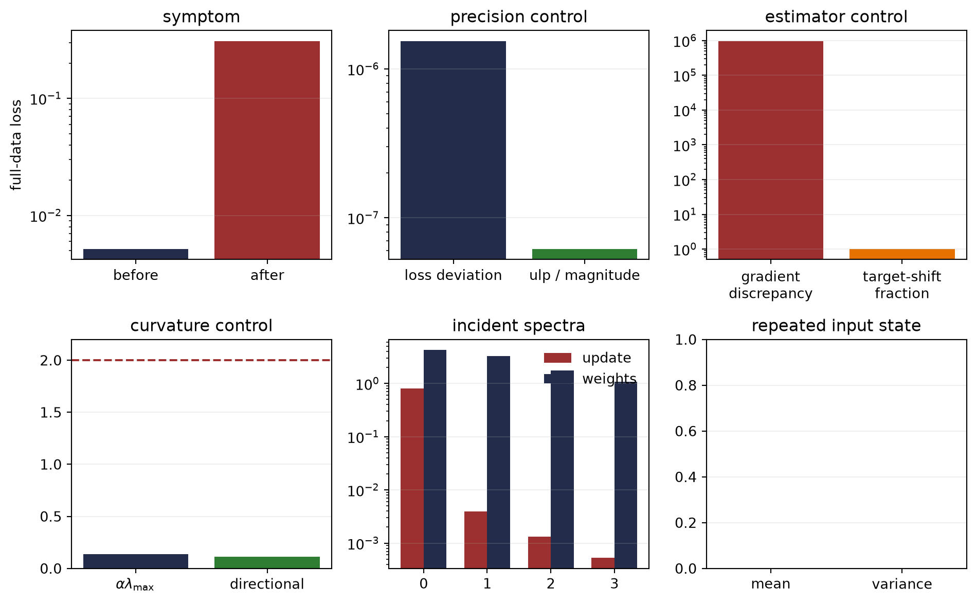
Figure Coda.1 — One engineered loss spike activates the complete diagnostic panel. Precision, curvature, and repeated-state controls acquit their named mechanisms; the update spectrum detects the event without explaining it; a same-input target control attributes \(99.8\%\) of the gradient discrepancy to the intervention. The panel diagnoses this pinned incident, not every loss spike.

The panels are not five votes. They are a sequence of attempts to falsify a cause.

Suspect 1: precision

The largest state or update magnitude is \(1.935\). The FP32 spacing at that scale is about \(1.19\times10^{-7}\). Across the complete paired trajectories, the maximum relative difference between float32 and float64 losses is only \(1.54\times10^{-6}\). Both runs exhibit the spike.

That does not prove the computation is numerically exact. It acquits range and local-grid resolution as explanations for a sixty-fold event in this run. A precision diagnosis has to predict the observed scale of the failure; here it does not.

Suspect 2: curvature

Because the displayed objective is linear least squares, its Hessian is constant. The top curvature is \(1.155\), so \(\alpha\lambda_{\max}=0.139\). The incident update’s directional value is \(\alpha\lambda_{\mathrm{dir}}=0.110\). Both remain far below the exact fixed-quadratic boundary at two.

C16 taught us not to use one local eigenvalue as a global theorem. This case is stronger: the landscape really is quadratic and its curvature does not move. The control predicts no curvature crossing, and none occurred.

Suspect 3: implementation state

Normalization state

The same eight input batches repeat every eight steps. The incident batch has the same coordinate means and variances as it had one cycle earlier: both maximum differences are exactly zero in the represented data. Any input normalizer using those declared statistics would receive the same state.

This does not acquit every stateful implementation. It eliminates the named rival: a changed input-statistic state at the incident step.

Update geometry

The leading update singular value is 176 times its value at the preceding step, and the incident update is nearly rank one. The spectrum therefore detects the event.

But detection is not diagnosis.

The current weight singular values remain broad, and nothing in the spectrum alone says whether the large direction came from curvature, data, arithmetic, or a routing bug.

C17’s instrument is a locator. It identifies which matrix and directions changed; it must be paired with a mechanism-specific control.

Suspect 4: estimator and data

At the incident step, the realized batch gradient differs from the clean full gradient by about \(9.74\times10^5\) times the squared full-gradient norm. More decisively, \(99.8\%\) of that discrepancy is reproduced by comparing the actual incident target with the clean target on the same input batch.

The sealed intervention can now be opened: at step 60, the four target coordinates in one batch were shifted by a fixed signed amount of magnitude eight. Inputs, batch order, step size, curvature, dtype, and normalization statistics were unchanged. This is not merely a high-variance draw under the declared clean estimator. Its conditional mean targets a different objective for one step.

Clipping the update could reduce the visible spike, but C13 already tells us what that repair would and would not do. It would bound the consequence while leaving the target violation unexplained. The correct incident response is to trace the batch target and its provenance.

Completed incident report

Field	Finding	Verdict
1. Symptom	full loss increases by \(60.2\times\) after step 60	established
2. Prediction	precision, curvature, estimator/data, and implementation state are predeclared rivals	each retains an acquitting control before the panel opens
3. Contract	seeded \(6\times4\) linear map; 256 observations; batch 32; step \(0.12\); fixed batch order	target, axes, denominator, dtype pair, seed, device, and wheel are declared
4. Precision control	paired FP32/FP64 loss deviation at most \(1.54\times10^{-6}\)	acquitted for this event
5. Curvature control	\(\alpha\lambda_{\max}=0.139\); directional value \(0.110\)	acquitted
6. Estimator control	\(99.8\%\) of gradient discrepancy traced to target shift	cause identified
7. Spectrum locator	leading update singular value jumps \(176\times\)	detects only
8. State control	repeated input-batch mean and variance unchanged	named normalization-state rival acquitted
9. Verdict	the step-60 batch targets a different objective	cause identified; precision, curvature, and named state rival acquitted
10. Corrective control	restore clean target; rerun same seed and batch order	spike removed by construction

A blank copy and three cumulative act assignments are in the final appendix. Its second incident is intentionally unrevealed and may remain unidentifiable under the supplied instruments.

The first page’s question now has an answer and a method. A loss trace proposes an incident; it does not name one. Geometry supplies candidate directions, dynamics supplies time-indexed boundaries, and the machine supplies arithmetic and state contracts. The estimator discipline binds them to the quantity the code actually computed.

That is what it means to make a training run diagnosable — and therefore trainable.