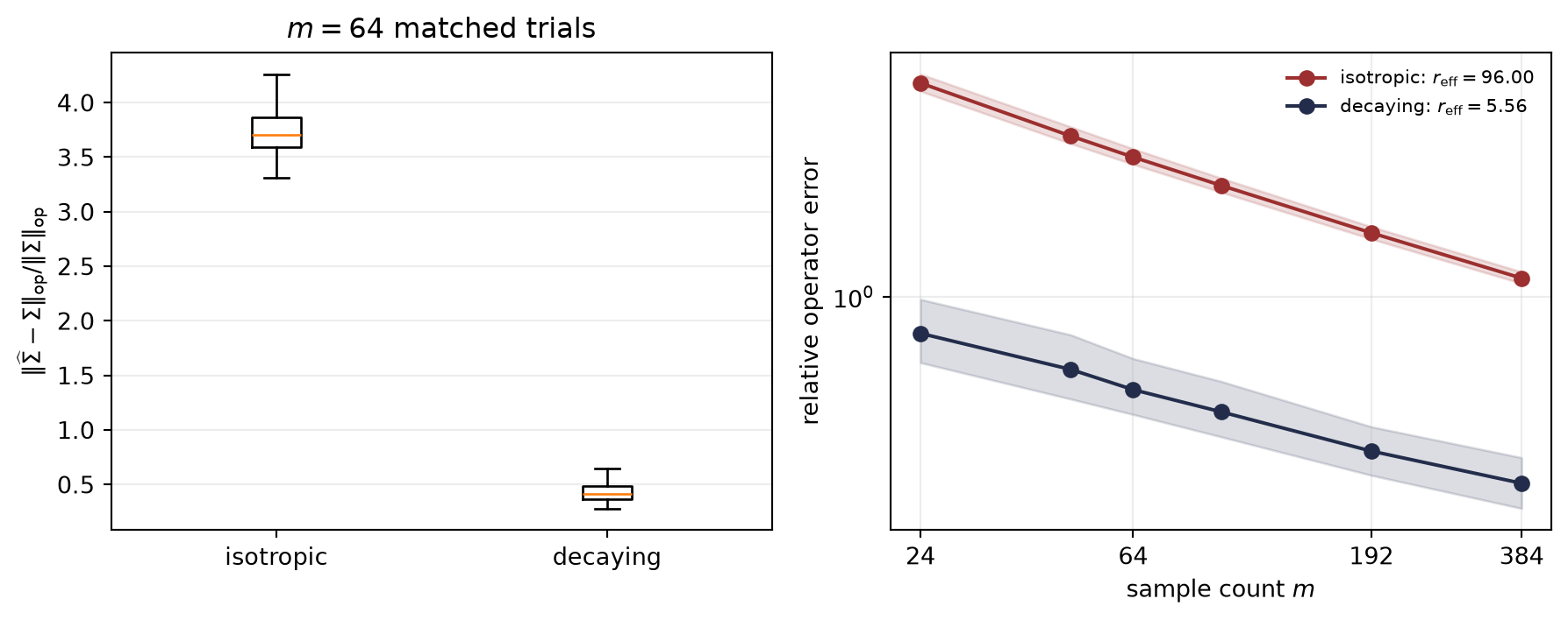
Consider two Gaussian populations in \(\mathbb{R}^{96}\). Both covariance matrices have algebraic rank \(96\). Both have operator norm one. Yet with only \(64\) observations, the median relative operator-norm error of the sample covariance is about \(3.71\) for one population and \(0.42\) for the other.
Nothing about rank or largest eigenvalue alone predicts this nine-fold difference. The missing quantity measures how much spectral mass sits below the leading direction.
ImportantPrediction
If two covariance matrices have the same dimension, rank, and largest eigenvalue, which remaining rival would you inspect first: condition number, determinant, a truncation rank, or the full decay profile? Name the scalar summary you would want that rival to justify.
Every diagonal entry in the second matrix is positive, so both matrices are full rank. Their leading eigenvalues are both one. The experiment below uses the same standard-normal draws for the two populations at every sample count; only the spectral coloring changes.
Load the chapter-pinned covariance instruments.
Construct the two full-rank population spectra.
Run the predeclared matched Gaussian covariance trials.
Compute relative operator-norm error quantiles.
Compare the \(m=64\) error distributions.
Trace the median and 10–90 percent bands across sample counts.
import matplotlib.pyplot as pltimport numpy as np# [1]from trainable_harness import ( effective_rank_psd, gaussian_covariance_error_trials,)# [2]dimension =96spectra = {"isotropic": np.ones(dimension),"decaying": 0.82** np.arange(dimension),}effective_ranks = { name: effective_rank_psd(np.diag(eigenvalues)).effective_rankfor name, eigenvalues in spectra.items()}# [3]sample_counts = np.array([24, 48, 64, 96, 192, 384])trial_count =300base_seed =int( sha256(b"c10-full-rank-few-directions").hexdigest()[:8],16,)errors = {name: {} for name in spectra}for sample_count in sample_counts: seed = (base_seed +int(sample_count)) % (2**32)for name, eigenvalues in spectra.items(): errors[name][sample_count] = gaussian_covariance_error_trials( eigenvalues,int(sample_count), trials=trial_count, seed=seed, )["relative_operator_error"]# [4]quantiles = { name: np.array([ np.quantile(errors[name][sample_count], [0.1, 0.5, 0.9])for sample_count in sample_counts ])for name in spectra}# [5]fig, axes = plt.subplots(1, 2, figsize=(9.4, 3.8))axes[0].boxplot( [errors["isotropic"][64], errors["decaying"][64]], tick_labels=["isotropic", "decaying"], showfliers=False,)axes[0].set( title="$m=64$ matched trials", ylabel=r"$\|\widehat{\Sigma}-\Sigma\|_{\mathrm{op}}/\|\Sigma\|_{\mathrm{op}}$",)axes[0].grid(axis="y", alpha=0.22)# [6]colors = {"isotropic": "#9C2F2F", "decaying": "#232D4B"}for name in spectra: q = quantiles[name] axes[1].plot( sample_counts, q[:, 1], marker="o", color=colors[name], label=rf"{name}: $r_{{\rm eff}}={effective_ranks[name]:.2f}$", ) axes[1].fill_between( sample_counts, q[:, 0], q[:, 2], color=colors[name], alpha=0.16, )axes[1].set( xscale="log", yscale="log", xlabel="sample count $m$", ylabel="relative operator error",)shown_counts = [24, 64, 192, 384]axes[1].set_xticks(shown_counts, labels=[str(value) for value in shown_counts])axes[1].minorticks_off()axes[1].grid(alpha=0.22)axes[1].legend(frameon=False, fontsize=8)plt.tight_layout()plt.show()print(f"harness={manifest['harness_ref']} wheel={manifest['wheel_sha256'][:12]}")for name in spectra:print(f"{name}: rank={np.linalg.matrix_rank(np.diag(spectra[name]))}, "f"operator_norm={spectra[name][0]:.1f}, "f"effective_rank={effective_ranks[name]:.6f}, "f"median_error_m64={np.median(errors[name][64]):.6f}" )
Figure 10.1: Rank and top eigenvalue do not determine covariance-estimation difficulty. Both 96-dimensional populations are full rank with operator norm one. Their effective ranks are 96 and about 5.56. Across 300 matched Gaussian trials, the decaying-spectrum covariance has far smaller relative operator-norm error.
The comparison does not say that decay makes every statistical problem easy. It isolates one claim: for operator-norm covariance estimation under this model, the spectral mass below the top eigenvalue changes the relevant dimension.
10.2 Replace the coordinate count by spectral mass
For a positive-semidefinite matrix \(\matr{\Sigma}\ne\matr{0}\), define its effective rank
It is the total spectral mass measured in units of the largest eigenvalue. The isotropic covariance spends one full unit in every direction, giving \(r_{\mathrm{eff}}=96\). The decaying spectrum spends \(\sum_{j=0}^{95}0.82^j\approx5.56\) such units.
Theorem 10.1 (Range and invariances of effective rank) For every nonzero positive-semidefinite \(\matr{\Sigma}\in\mathbb{R}^{n\times n}\),
\[
1
\le
r_{\mathrm{eff}}(\matr{\Sigma})
\le
\operatorname{rank}(\matr{\Sigma})
\le n.
\tag{10.4}\]
Moreover, effective rank is unchanged by positive scalar rescaling and by orthogonal change of coordinates.
Proof
Let the positive eigenvalues be \(\lambda_1\ge\cdots\ge\lambda_r>0\). Because the trace includes \(\lambda_1\),
Because every positive eigenvalue is at most \(\lambda_1\),
\[
\frac{\sum_{j=1}^r\lambda_j}{\lambda_1}\le r.
\]
Multiplying \(\matr{\Sigma}\) by \(c>0\) multiplies numerator and denominator by \(c\). Orthogonal similarity preserves the eigenvalues, hence both trace and operator norm. \(\square\)
Algebraic rank changes only when an eigenvalue becomes exactly zero. Effective rank changes continuously as spectral mass moves.
WarningNamed wrong answer: effective rank is stable rank
The notions are related, but they apply to different objects. For a general matrix \(\matr{A}\), stable rank is \(\norm{\matr{A}}_{\mathrm F}^2/\norm{\matr{A}}_{\mathrm{op}}^2\). For a covariance \(\matr{\Sigma}\), that expression is \(\sum_j\lambda_j^2/\lambda_1^2\), not \(\sum_j\lambda_j/\lambda_1\).
Theorem 10.2 (Stable rank is effective rank after squaring) For every nonzero real matrix \(\matr{A}\),
The trace of \(\matr{A}^{\mathsf T}\matr{A}\) is \(\norm{\matr{A}}_{\mathrm F}^2\), while its operator norm is \(\norm{\matr{A}}_{\mathrm{op}}^2\). Substitute these identities into Equation 10.3. \(\square\)
This identity is the safe bridge between the terms. It does not license swapping them on the same matrix.
10.3 Why this quantity enters covariance error
Write the estimation error as an average of centered random matrices:
C06 warned that squaring a sub-Gaussian quantity changes the concentration class. Covariance estimation is exactly that operation, simultaneously over all directions. C07 supplied the finite approximation of the sphere, and C08 identified the operator norm as the worst directional error. Effective rank records the matrix variance scale left after those steps.
Theorem 10.3 (Gaussian covariance summand) If \(\vect{x}\sim\mathcal{N}(\vect{0},\matr{\Sigma})\), then
Work in an eigenbasis and write \(x_j=\sqrt{\lambda_j}g_j\) with independent standard-normal \(g_j\). The \((j,k)\) entry of \(\mathbb{E}[\vect{x}\vect{x}^{\mathsf T}\vect{x}\vect{x}^{\mathsf T}]\) is \(\mathbb{E}[x_jx_k\sum_\ell x_\ell^2]\). For \(j\ne k\), symmetry makes this zero. For \(j=k\), Gaussian fourth moments give
Thus \(\mathbb{E}[(\vect{x}\vect{x}^{\mathsf T})^2]
=\operatorname{tr}(\matr{\Sigma})\matr{\Sigma}
+2\matr{\Sigma}^2\). Expanding the centered square subtracts one copy of \(\matr{\Sigma}^2\). \(\square\)
The coordinate dimension has disappeared from this variance expression. It re-enters when the spectrum actually distributes mass across that many directions.
10.4 A usable covariance theorem
Theorem 10.4 (Effective-rank covariance bound) Let \(\vect{x}_1,\ldots,\vect{x}_m\) be independent copies of a mean-zero random vector with covariance \(\matr{\Sigma}\). Assume that for every \(\vect{u}\),
The proof symmetrizes the empirical process, controls a quadratic process indexed by the sphere, and converts its complexity to effective rank. That chain requires machinery beyond this chapter’s diagnostic target. See Vershynin’s second-edition Theorem 9.2.2 (Vershynin 2026) for a nonasymptotic derivation and Koltchinskii and Lounici (2017) for sharp effective-rank formulations.
Diagnostic proof sketch
The pointer hides technical machinery, not the causal route. First, symmetrization replaces the centered empirical error by a signed quadratic process:
where the signs \(\varepsilon_i\) are independent of the observations. Second, C06’s square warning identifies the fixed-\(\vect u\) object as sub-exponential rather than sub-Gaussian. Third, C07’s finite-cover move turns fixed directions into a uniform operator statement.
A crude Euclidean net pays ambient dimension and loses the point of this chapter. The refined argument measures the ellipsoid \(\matr\Sigma^{1/2}S^{n-1}\) in its covariance metric. Its squared average radius is \(\operatorname{tr}(\matr\Sigma)\) and its largest squared radius is \(\norm{\matr\Sigma}_{\mathrm{op}}\); their ratio is exactly \(r_{\mathrm{eff}}\). Chaining or a matrix-deviation theorem carries that anisotropic geometry through the supremum and produces the \(\sqrt{r_{\mathrm{eff}}/m}+r_{\mathrm{eff}}/m\) scale. The pointer supplies that final uniform-process step; the sketch explains why effective rank, and not algebraic rank alone, is the complexity that enters.
The usable scaling is \(m\gg r_{\mathrm{eff}}(\matr{\Sigma})\). Dimension has not been abolished; it has been replaced by a spectrum-sensitive complexity under explicit tail assumptions.
TipField note: one scalar is not a compression budget
Effective rank does not say how many coordinates may be deleted at a chosen error tolerance. It does not identify important eigenvectors, certify a low-rank approximation, or explain why a trained model generalizes. Those questions require information this scalar discards.
squared singular mass relative to the top singular value
truncation rank
how many directions meet a declared tolerance?
task-dependent compression
The table prevents a rhetorical slide: observing a small effective rank and then speaking as though a compression guarantee or generalization theorem had been proved.
10.6 The Act I handoff
Act I began with a safe zone for one random projection. It followed squares into a two-regime tail, paid for a finite cover, measured both singular edges, calibrated an empirical spectral bulk, and replaced nominal dimension by a spectrum-sensitive complexity.
The next act changes the moving object. Instead of asking what a random matrix looks like, we ask how derivatives move backward through a computation and what state the machine must retain to make that motion possible.
NoteCheck yourself
A covariance has eigenvalues \((1,1/2,1/4,1/8)\). Compute its algebraic rank, effective rank, and stable rank when the covariance itself is treated as the matrix. Then compute the stable rank of a square root \(\matr{A}\) satisfying \(\matr{A}^{\mathsf T}\matr{A}=\matr{\Sigma}\). Which two quantities agree?
10.7 Okay, so —
Inherited: operator norm asks for the worst direction; empirical spectra require a finite null; squares leave the sub-Gaussian safe zone.
Changed: nominal coordinate count became total spectral mass measured in top-eigenvalue units.
Instrumented: matched Gaussian trials separated two full-rank covariances with the same operator norm.
Established: effective rank controls the diagnostic sample scale for covariance estimation under a relative sub-Gaussian contract.
Unresolved: How does derivative information traverse a computation when a scalar spectrum summary cannot say which paths matter?
10.8 Sources and further reading
The effective/stable-rank identity is recorded in Vershynin’s second-edition Remark 5.6.4, and the covariance theorem is Theorem 9.2.2 (Vershynin 2026). Sharp expectation and high-probability bounds are developed by Koltchinskii and Lounici (2017). The warning that effective dimension alone does not imply generalization is consistent with the interpolation evidence of Zhang et al. (2017).
For the general theory, use Vershynin (2026) and Koltchinskii and Lounici (2017); this chapter’s contribution is the full-rank/few-directions witness and the separation of five dimension summaries.
Reading order. Start with Vershynin (2026) for the book’s exact notation and the covariance theorem, then read Koltchinskii and Lounici (2017) for sharper bounds and Zhang et al. (2017) for the boundary on generalization claims.
10.9 Exercises
(Pencil.) Prove that \(r_{\mathrm{eff}}(\matr{\Sigma})=n\) for a nonzero \(n\times n\) positive-semidefinite matrix if and only if all eigenvalues are equal.
(Code.) Replace \(0.82\) in Equation 10.2 by values from \(0.5\) to \(0.99\). Plot median relative operator error against effective rank at a fixed sample count. Keep the matched-randomness contract.
(Audit.) A paper reports “the representation is effectively ten-dimensional” from a scalar effective-rank estimate. List three claims that do not follow and name the missing evidence for each.
(Audit.) Paper audit: Complete the Mathematical object, Evidence culture and interface, Assumption stress test, Discriminating control, and Transfer verdict fields of the Paper Autopsy Protocol. Identify the matrix, centering and scaling convention, effective-rank definition, and target conclusion. Does the cited theorem support that conclusion?
(Pencil.) Construct two six-dimensional spectra with the same operator norm and effective rank but different truncation ranks at relative tolerance \(0.1\). State which covariance claim remains comparable and which compression claim changes.
(Audit.) Act checkpoint — extend the Incident Card. Complete the Act I assignment. Add a named matrix, finite-null or perturbation control, and a “detects only” option to the Act 0 card. Route: Act checkpoint. Estimated time: 75 minutes. Deliverable: the revised card and one spectrum plot whose matrix is named in the caption. Hint: plotting the wrong matrix can produce a true spectrum and a false diagnosis.
Koltchinskii, Vladimir, and Karim Lounici. 2017. “Concentration Inequalities and Moment Bounds for Sample Covariance Operators.”Bernoulli 23 (1): 110–33. https://doi.org/10.3150/15-BEJ730.
Vershynin, Roman. 2026. High-Dimensional Probability: An Introduction with Applications in Data Science. 2nd ed. Cambridge Series in Statistical and Probabilistic Mathematics. Cambridge University Press. https://www.math.uci.edu/~rvershyn/papers/HDP-book/HDP-book.html.
Zhang, Chiyuan, Samy Bengio, Moritz Hardt, Benjamin Recht, and Oriol Vinyals. 2017. “Understanding Deep Learning Requires Rethinking Generalization.”International Conference on Learning Representations. https://openreview.net/forum?id=Sy8gdB9xx.