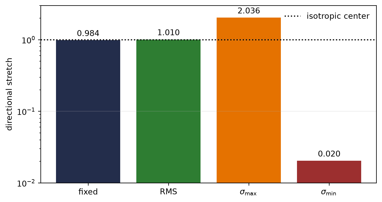
8 One Average, Two Edges: Random Operators and Singular Values

RS · Random-matrix spectra SG · The sub-Gaussian safe zone Geometric primary · Dynamic quiet · Algorithmic supporting

Draw a \(64\times64\) matrix \(\matr{A}\) with independent \(\mathcal{N}(0,1/64)\) entries. Before seeing it, choose the first coordinate vector \(\vect{e}_1\). In the seeded realization below,

\[ \norm{\matr{A}\vect{e}_1}_2\approx0.984, \qquad \frac{\norm{\matr{A}}_{\mathrm{F}}^2}{64}\approx1.019. \]

Both checks say “near one.” The same matrix has largest singular value about \(2.036\) and smallest singular value about \(0.0204\). Its most contracted direction loses nearly two orders of magnitude relative to its most stretched direction.

Prediction

For every fixed unit vector \(\vect{x}\), \(\E\norm{\matr{A}\vect{x}}_2^2=1\). Which word in that statement prevents it from proving that the realized matrix preserves every direction? What diagnostic replaces the expectation when the direction is chosen after the matrix is observed?

8.1 The direction can adapt to the matrix

The top and bottom singular vectors are functions of the realized matrix. They are not fixed anchors to which one may apply a single-direction concentration statement. C07 built the missing route from fixed anchors to adaptive extrema; this chapter gives those extrema names and instruments.

Load the chapter-pinned operator instruments.
Generate one scaled Gaussian matrix from a declared seed.
Compare a predeclared direction and the Frobenius average with exact SVD edges.
Verify the stretches of the top and bottom right singular vectors.
Plot the average checks beside the adaptive edges.

import matplotlib.pyplot as plt
import numpy as np

# [1]

from trainable_harness import (
    gaussian_singular_value_trials,
    matrix_spectrum_summary,
    power_iteration_spectral_norm,
)

# [2]
dimension, matrix_seed = 64, 6224
rng = np.random.default_rng(matrix_seed)
matrix = rng.standard_normal((dimension, dimension)) / np.sqrt(dimension)

# [3]
summary = matrix_spectrum_summary(matrix)
fixed_direction = np.zeros(dimension)
fixed_direction[0] = 1.0
fixed_stretch = np.linalg.norm(matrix @ fixed_direction)
root_mean_squared_stretch = np.sqrt(summary.mean_squared_stretch)

# [4]
_, singular_values, right_vectors_t = np.linalg.svd(
    matrix,
    full_matrices=False,
)
top_stretch = np.linalg.norm(matrix @ right_vectors_t[0])
bottom_stretch = np.linalg.norm(matrix @ right_vectors_t[-1])
assert np.isclose(top_stretch, summary.sigma_max)
assert np.isclose(bottom_stretch, summary.sigma_min)
assert np.allclose(singular_values, np.asarray(summary.singular_values))

# [5]
labels = ["fixed", "RMS", r"$\sigma_{\max}$", r"$\sigma_{\min}$"]
values = [
    fixed_stretch,
    root_mean_squared_stretch,
    summary.sigma_max,
    summary.sigma_min,
]
fig, axis = plt.subplots(figsize=(6.9, 3.7))
bars = axis.bar(labels, values, color=["#232D4B", "#2E7D32", "#E57200", "#9C2F2F"])
axis.axhline(1.0, color="black", linestyle=":", label="isotropic center")
axis.set(ylabel="directional stretch", yscale="log", ylim=(0.01, 3.0))
axis.grid(alpha=0.25, axis="y")
axis.legend(frameon=False)
axis.bar_label(bars, fmt="%.3f", padding=3)
plt.tight_layout()
plt.show()

print(f"harness={manifest['harness_ref']} wheel={manifest['wheel_sha256'][:12]}")
print(
    f"fixed={fixed_stretch:.6f}; "
    f"mean squared={summary.mean_squared_stretch:.6f}"
)
print(
    f"sigma_max={summary.sigma_max:.6f}; "
    f"sigma_min={summary.sigma_min:.6f}; "
    f"kappa={summary.condition_number:.3f}"
)

Bar chart on a logarithmic vertical scale. Fixed-direction stretch and root-mean-squared stretch are near one, the largest singular value is about two, and the smallest singular value is near 0.02. — Figure 8.1: One average conceals two adaptive edges. For the seeded square Gaussian matrix, the predeclared coordinate direction and root-mean-squared directional stretch sit near one. The top singular direction stretches by about two, while the bottom singular direction nearly collapses. Exact SVD is the control; this one matrix is a witness, not an asymptotic law.

harness=ch-08 wheel=9ec8176699a4
fixed=0.984012; mean squared=1.019185
sigma_max=2.036060; sigma_min=0.020407; kappa=99.773

This phenomenon does not contradict isotropy. For a fixed unit vector,

\[ \E\norm{\matr{A}\vect{x}}_2^2 = \sum_{i=1}^{m} \E\langle\vect{a}_i,\vect{x}\rangle^2 =1 \tag{8.1}\]

under the \(1/\sqrt m\) scaling. The quantifiers are:

\[ \text{for each fixed }\vect{x}, \quad \E_{\matr{A}}[\cdots]=1. \]

They are not:

\[ \text{for each realized }\matr{A}, \quad \text{for every }\vect{x},\ [\cdots]=1. \]

Moving “every direction” through the random draw is exactly the uniformization problem.

8.2 Two edges define the stretch interval

For \(\matr{A}\in\mathbb{R}^{m\times n}\) with \(m\ge n\), write the singular value decomposition

\[ \matr{A} = \matr{U}\matr{\Sigma}\matr{V}^{\mathsf T}, \qquad \sigma_1\ge\cdots\ge\sigma_n\ge0. \tag{8.2}\]

We use

\[ \sigma_{\max}(\matr{A})=\sigma_1, \qquad \sigma_{\min}(\matr{A})=\sigma_n, \qquad \norm{\matr{A}}_{\mathrm{op}}=\sigma_{\max}(\matr{A}). \]

Theorem 8.1 (Singular-value stretch interval) For every \(\vect{x}\in\mathbb{R}^n\),

\[ \sigma_{\min}(\matr{A})\norm{\vect{x}}_2 \le \norm{\matr{A}\vect{x}}_2 \le \sigma_{\max}(\matr{A})\norm{\vect{x}}_2. \tag{8.3}\]

Both inequalities are attained at the corresponding right singular vectors.

Proof

Put \(\vect{z}=\matr{V}^{\mathsf T}\vect{x}\). Orthogonality preserves the Euclidean norm, so \(\norm{\vect{z}}_2=\norm{\vect{x}}_2\) and

\[ \norm{\matr{A}\vect{x}}_2^2 = \norm{\matr{\Sigma}\vect{z}}_2^2 = \sum_{j=1}^{n}\sigma_j^2z_j^2. \]

Bounding every \(\sigma_j^2\) between \(\sigma_n^2\) and \(\sigma_1^2\) proves Equation 8.3. Choosing \(\vect{x}\) as the first or last column of \(\matr{V}\) gives equality. \(\square\)

The Frobenius norm measures a different summary:

\[ \norm{\matr{A}}_{\mathrm{F}}^2 = \sum_{j=1}^{n}\sigma_j^2, \qquad \frac{\norm{\matr{A}}_{\mathrm{F}}^2}{n} = \text{mean squared singular value}. \tag{8.4}\]

The average can equal one while the interval is wide. An exact isometry has every singular value equal to one. This is the first entry in the book’s orthogonality/scale ledger.

Named wrong answer: ‘Small singular value means underflow’

A singular value is a relative geometric scale. Underflow is an absolute arithmetic event determined by input magnitude, subsequent operations, dtype, and storage/accumulation rules. A small lower edge predicts directional suppression; it does not, by itself, say that any represented number becomes subnormal or zero.

8.3 From fixed rows to all directions

Let the unscaled rows \(\vect{a}_i\in\mathbb{R}^n\) be independent, centered, isotropic, and sub-Gaussian. For each fixed unit vector \(\vect{x}\), \(\langle\vect{a}_i,\vect{x}\rangle\) lies in C05’s safe zone. The squared quantity

\[ \norm{\matr{A}\vect{x}}_2^2 = \sum_{i=1}^{m} \langle\vect{a}_i,\vect{x}\rangle^2 \]

lies in C06’s sub-exponential regime. Bernstein controls this sum at one fixed direction. A C07 net and a deterministic quadratic-form interpolation then extend the result over the sphere.

Theorem 8.2 (Two-sided sub-Gaussian matrix bound) Let \(\matr{A}\) have independent, centered, isotropic, sub-Gaussian rows, and let

\[ K=\max_i\norm{\vect{a}_i}_{\psi_2}. \]

There is a universal constant \(C>0\) such that, for every \(t\ge0\), with probability at least \(1-2e^{-t^2}\),

\[ \sqrt m-CK^2(\sqrt n+t) \le \sigma_{\min}(\matr{A}) \le \sigma_{\max}(\matr{A}) \le \sqrt m+CK^2(\sqrt n+t). \tag{8.5}\]

Diagnostic proof sketch

For fixed \(\vect{x}\), isotropy centers \(m^{-1}\norm{\matr{A}\vect{x}}_2^2\) at one. C06 turns each centered square into a sub-exponential variable, so Bernstein bounds its deviation. Choose a constant-radius net with exponentially many anchors, and let the exponent pay the log covering cost from C07. Apply the symmetric quadratic-form version of the net interpolation to

\[ \frac{1}{m}\matr{A}^{\mathsf T}\matr{A}-\matr{I}. \]

The resulting operator-norm control bounds every eigenvalue of the Gram matrix, hence every squared singular value. Careful conversion from squared edges to singular edges gives Equation 8.5. Vershynin supplies the constant bookkeeping (Vershynin 2026).

This proof anatomy is more important diagnostically than the unnamed universal constant:

Ingredient	Contribution
isotropy	center at \(\sqrt m\) before scaling
sub-Gaussian row projections	fixed-direction tail
squaring plus Bernstein	concentration of directional energy
sphere cover	\(\sqrt n\) uniformization cost
interpolation	all directions between anchors

The lower statement becomes informative only when its displayed lower bound is positive. For a nearly square matrix, the generic theorem may correctly refuse to certify a margin.

8.4 Aspect ratio opens the lower edge

Gaussian matrices admit a sharper benchmark. The sharp constants require Gaussian comparison, not merely the elementary net calculation.

Theorem 8.3 (Gaussian singular-edge benchmark) Let \(\matr{G}\in\mathbb{R}^{m\times n}\), \(m\ge n\), have independent standard-normal entries. Then

\[ \E\sigma_{\max}(\matr{G}) \le \sqrt m+\sqrt n, \qquad \E\sigma_{\min}(\matr{G}) \ge \sqrt m-\sqrt n. \tag{8.6}\]

Gaussian concentration gives sub-Gaussian upper and lower deviations around these edge locations. After scaling \(\matr{A}=\matr{G}/\sqrt m\), the benchmark interval is

\[ 1-\sqrt{\frac{n}{m}} \quad\text{to}\quad 1+\sqrt{\frac{n}{m}}. \tag{8.7}\]

Proof with pointer

The upper expectation is a supremum of the Gaussian process \(\langle\matr{G}\vect{x},\vect{y}\rangle\) over two unit spheres. The lower edge is the corresponding min–max process. Gaussian comparison bounds them by sums and differences of Gaussian-vector norms; Gaussian concentration then supplies deviations. This chapter uses the result as a diagnostic benchmark. The comparison proof is given in Vershynin (Vershynin 2026).

For \(m=n\), the lower benchmark is zero. It does not say that every finite square Gaussian matrix is singular. It says that this theorem supplies no dimension-independent positive lower margin. The opening realization’s condition number near \(99.8\) is therefore not evidence against isotropy.

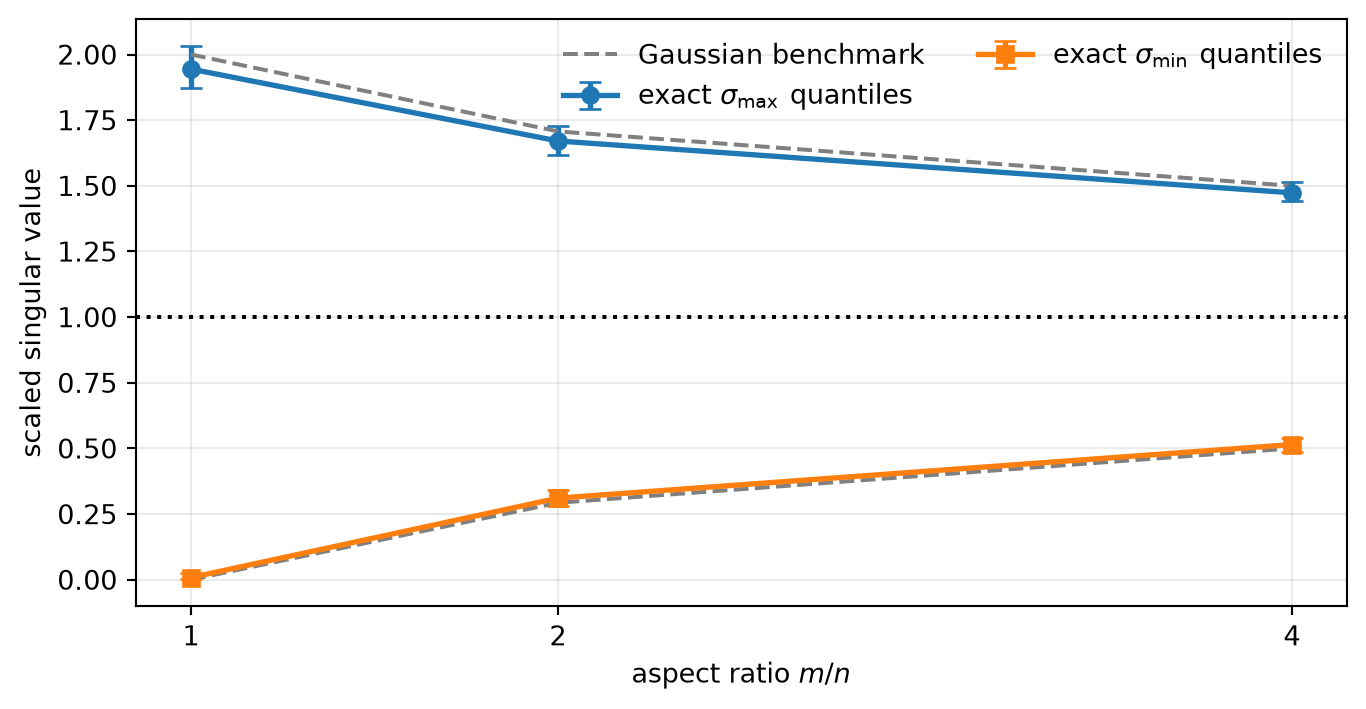
The next study holds \(n=64\) fixed and increases \(m\). Every point is computed from exact SVDs of \(160\) independently seeded finite matrices. The curves in Equation 8.7 are benchmarks, not fitted parameters and not an empirical spectral-density theorem.

Fix the input dimension and a grid of row counts.
Generate independent scaled Gaussian matrices for each shape.
Compute exact upper and lower singular edges for every trial.
Report predeclared 5th, 50th, and 95th percentiles.
Compare the finite ensembles with the aspect-ratio benchmark.

# [1]
columns = 64
rows_grid = np.array([64, 128, 256])
trials = 160

# [2]
ensembles = [
    gaussian_singular_value_trials(
        int(rows),
        columns,
        trials=trials,
        seed=6225 + index,
    )
    for index, rows in enumerate(rows_grid)
]

# [3]
lower = np.array([np.median(item["sigma_min"]) for item in ensembles])
upper = np.array([np.median(item["sigma_max"]) for item in ensembles])
lower_interval = np.array(
    [
        [np.quantile(item["sigma_min"], 0.05), np.quantile(item["sigma_min"], 0.95)]
        for item in ensembles
    ]
)
upper_interval = np.array(
    [
        [np.quantile(item["sigma_max"], 0.05), np.quantile(item["sigma_max"], 0.95)]
        for item in ensembles
    ]
)

# [4]
lower_error = np.vstack((lower - lower_interval[:, 0], lower_interval[:, 1] - lower))
upper_error = np.vstack((upper - upper_interval[:, 0], upper_interval[:, 1] - upper))

# [5]
ratios = rows_grid / columns
benchmark_lower = 1.0 - 1.0 / np.sqrt(ratios)
benchmark_upper = 1.0 + 1.0 / np.sqrt(ratios)
fig, axis = plt.subplots(figsize=(7.2, 3.8))
axis.errorbar(
    ratios,
    upper,
    yerr=upper_error,
    fmt="o-",
    capsize=4,
    linewidth=2.0,
    label=r"exact $\sigma_{\max}$ quantiles",
)
axis.errorbar(
    ratios,
    lower,
    yerr=lower_error,
    fmt="s-",
    capsize=4,
    linewidth=2.0,
    label=r"exact $\sigma_{\min}$ quantiles",
)
axis.plot(ratios, benchmark_upper, "--", color="gray", label="Gaussian benchmark")
axis.plot(ratios, benchmark_lower, "--", color="gray")
axis.axhline(1.0, color="black", linestyle=":")
axis.set(
    xlabel=r"aspect ratio $m/n$",
    ylabel="scaled singular value",
    xticks=ratios,
)
axis.grid(alpha=0.25)
axis.legend(frameon=False, ncol=2)
plt.tight_layout()
plt.show()

for rows, lo, hi in zip(rows_grid, lower, upper, strict=True):
    print(
        f"shape={rows}x{columns}: "
        f"median sigma_min={lo:.6f}, median sigma_max={hi:.6f}"
    )

Plot of singular value versus row-to-column ratio one, two, and four. Median largest singular values decrease from about 1.94 to 1.47, while median smallest singular values increase from about 0.008 to 0.515. Error bars show fifth and ninety-fifth percentiles, and dashed benchmark curves follow one plus or minus the inverse square root of the row-to-column ratio. — Figure 8.2: Aspect ratio changes the margin between singular edges. Exact SVD quantiles from 160 finite Gaussian matrices per shape move toward the scaled Gaussian benchmark as the row count grows relative to the fixed input width. The square case has no positive lower benchmark; taller maps open one. Error bars show empirical fifth-to-ninety-fifth percentile ranges, not confidence intervals for a population edge.

shape=64x64: median sigma_min=0.008079, median sigma_max=1.944530
shape=128x64: median sigma_min=0.310570, median sigma_max=1.670645
shape=256x64: median sigma_min=0.514655, median sigma_max=1.473261

The median lower edge rises from about \(0.0081\) in the square ensemble to \(0.515\) at aspect ratio four. Meanwhile, the fixed-direction squared stretch and the mean squared singular value remain centered near one. “Preserves scale on average” and “has a positive uniform margin” are different claims.

8.5 One-sided instruments answer one-sided questions

Exact SVD is appropriate for these laptop controls, but expensive for a large matrix. Power iteration repeatedly applies \(\matr{A}^{\mathsf T}\matr{A}\):

\[ \vect{v}_{k+1} = \frac{ \matr{A}^{\mathsf T}\matr{A}\vect{v}_k }{ \norm{\matr{A}^{\mathsf T}\matr{A}\vect{v}_k}_2 }. \tag{8.8}\]

When the initialization has a component in the top right singular direction and the top eigenvalue is separated, the iteration amplifies that component. The estimate \(\norm{\matr{A}\vect{v}_k}_2\) approaches \(\sigma_{\max}(\matr{A})\).

Reuse the seeded matrix with an exact SVD control.
Initialize one unit vector from a separate declared seed.
Apply power iteration to the Gram operator.
Record the upper-edge estimate at every iteration.
Plot relative error and state which edge the instrument never queried.

# [1]
exact_upper = summary.sigma_max
exact_lower = summary.sigma_min

# [2]
iteration_seed, iterations = 6228, 25

# [3]
trace = power_iteration_spectral_norm(
    matrix,
    iterations=iterations,
    seed=iteration_seed,
)

# [4]
estimates = np.asarray(trace.estimates)
relative_error = np.abs(estimates - exact_upper) / exact_upper
assert relative_error[-1] < relative_error[0]

# [5]
fig, axis = plt.subplots(figsize=(6.9, 3.6))
axis.semilogy(
    np.arange(1, iterations + 1),
    relative_error,
    "o-",
    markersize=3.5,
    linewidth=2.0,
)
axis.set(
    xlabel="power iteration",
    ylabel=r"relative error in $\sigma_{\max}$",
)
axis.grid(alpha=0.25, which="both")
axis.text(
    0.98,
    0.94,
    rf"$\sigma_{{\min}}={exact_lower:.4f}$ was not queried",
    transform=axis.transAxes,
    ha="right",
    va="top",
)
plt.tight_layout()
plt.show()

print(
    f"first estimate={estimates[0]:.6f}; "
    f"last estimate={estimates[-1]:.6f}; "
    f"exact sigma_max={exact_upper:.6f}"
)
print(f"exact sigma_min={exact_lower:.6f}; power-iteration estimate=not produced")

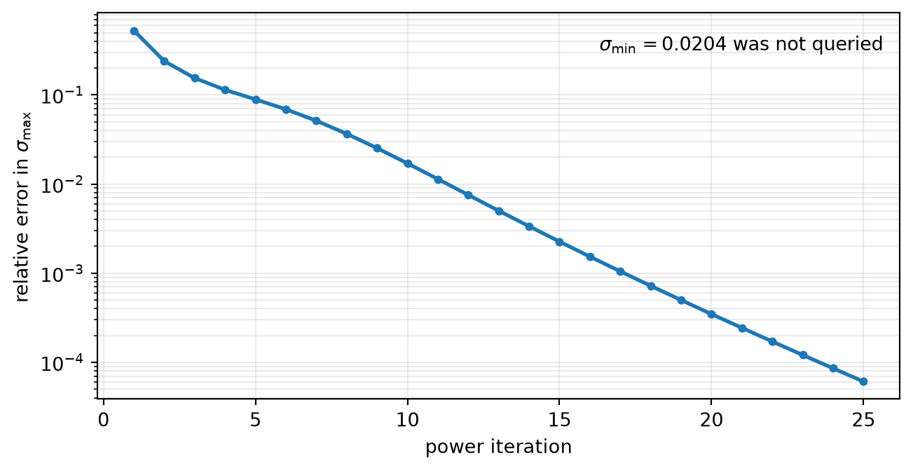
Semilog plot of relative error in the largest singular value estimate over 25 power iterations. Error decreases from order one toward below one ten-thousandth. An annotation states that the smallest singular value, about 0.0204, was not queried. — Figure 8.3: Power iteration is an upper-edge instrument. On the seeded control matrix, the estimate approaches the exact largest singular value over 25 iterations. The exact smallest singular value is shown only as a separate SVD control; it is not estimated by this trajectory. Convergence here validates the implementation on one matrix, not a universal iteration count.

first estimate=0.960212; last estimate=2.035936; exact sigma_max=2.036060
exact sigma_min=0.020407; power-iteration estimate=not produced

Power iteration controls the largest singular value only. Applying the same routine longer does not turn it into a lower-edge diagnostic. The smallest edge requires a different method—often an inverse or shifted procedure—and that procedure has its own conditioning and linear-solve contract.

Field note: keep an exact small control

At production scale, randomized or iterative estimators may be necessary. Before trusting them, run the identical code path on matrices small enough for an exact SVD. Record the stopping rule, iteration count, initialization, and spectral-gap sensitivity. An approximate instrument without a control can confuse estimator failure with a changing matrix.

The boundary between lenses is now explicit:

Observation	What it diagnoses	What remains missing
small \(\sigma_{\min}\)	relative directional suppression	absolute activation/gradient scale and dtype
large \(\sigma_{\max}\)	relative directional amplification	nonlinearities and trajectory
wide singular interval	poor realized isometry	whether products across depth worsen or cancel it
power estimate	upper edge under an iteration contract	lower edge and full spectral mass

C03 decides when an absolute represented value is unsafe. C14 will decide how singular intervals compose across depth. C09 asks the question omitted here: how is the spectral mass distributed between the two edges?

Check yourself

A scaled random matrix satisfies \(\norm{\matr{A}}_{\mathrm{F}}^2/n=1\) exactly, and a power iteration estimates \(\sigma_{\max}=1.8\). Can you bound \(\sigma_{\min}\) away from zero from those two numbers alone? Construct a set of singular values with the same Frobenius average and upper edge but an arbitrarily small lower edge.

8.6 Okay, so —

Inherited: C05 controlled fixed sub-Gaussian projections, C06 controlled their squares, and C07 supplied the finite-cover route to adaptive extrema.
Changed: the diagnostic target is a realized random operator, so a fixed expectation or Frobenius average no longer stands in for all directions.
Instrumented: the harness now reports exact singular summaries, seeded aspect-ratio ensembles, and a power-iteration trace validated against exact SVD.
Established: singular values bound every directional stretch; isotropy sets a fixed-direction center; concentration plus covering creates a dimension-dependent edge interval; aspect ratio controls whether the Gaussian lower benchmark has positive margin.
Unresolved: What does the spectral mass between two random-matrix edges say, and when does a finite outlier carry evidence rather than noise?

8.7 Sources and further reading

Vershynin develops the singular-value identities, two-sided sub-Gaussian matrix theorem, and Gaussian comparison bounds used here (Vershynin 2026). Miyato, Kataoka, Koyama, and Yoshida use power iteration inside an upper-edge intervention (Miyato et al. 2018); the paper supplies a useful audit of what such an instrument controls and what it leaves unmeasured.

For the general theory, use Vershynin (2026); this chapter’s contribution is the matched two-edge witness and its finite certificate boundary.

Reading order. Start with Vershynin (2026) for the two-edge theorem and its covering proof, then use Miyato et al. (2018) to audit what an upper-edge intervention does not say about the lower edge.

8.8 Exercises

(Pencil.) Same average, different interval. Construct two diagonal \(4\times4\) matrices with equal Frobenius norm and unequal operator norm. Then make the second matrix’s smallest singular value arbitrarily close to zero while preserving its Frobenius norm.
(Pencil.) Shape is part of the theorem. For a wide matrix \(\matr{A}\in\mathbb{R}^{m\times n}\) with \(m<n\), prove that its action on the full input space has lower edge zero. Explain why NumPy’s list of \(\min(m,n)\) returned singular values can obscure this nullspace if the shape contract is omitted.
(Code.) Fixed versus adaptive directions. Repeat the opening study for dimensions \(16\), \(64\), and \(256\). Predeclare ten unit directions before each matrix draw. Compare their largest stretch with exact singular edges, reporting seeds, trial denominators, and empirical quantiles.
(Code.) Instrument sensitivity. Build diagonal matrices with controlled ratios \(\sigma_2/\sigma_1\). Measure the iterations required for power iteration to reach a fixed relative error over many initializations. Relate failures to the starting component in the top direction.
(Audit.) Geometry is not arithmetic. A report observes \(\sigma_{\min}=10^{-4}\) and declares that gradients underflow in FP16. List the missing absolute-scale, operation, storage, and accumulation facts. Design the smallest dtype-aware experiment that could support the narrower arithmetic claim.
(Audit.) Paper audit: an upper-edge intervention. Complete the Mathematical object, Evidence culture and interface, Numerical and hardware contract, Discriminating control, and Transfer verdict fields for Miyato, Kataoka, Koyama, and Yoshida (Miyato et al. 2018). Extract the target singular quantity, the power-iteration approximation, the persistence of its auxiliary vectors, and the empirical stability endpoint. State precisely what the method controls, then identify why that evidence does not imply a positive lower singular edge or a bounded condition number.