2 One Pass, Two Failures: Streaming State and Stable Variance

NS · Numerical stability Geometric quiet · Dynamic quiet · Algorithmic primary

A variance cannot be negative. Yet the following one-pass calculation returns one.

An impossible output is more than a failed test: it is a diagnostic instrument.

It tells us that algebraic correctness did not survive execution.

The setting is ordinary. We receive a stream \(x_1,\ldots,x_n\), and we want its population variance

\[ \sigma_n^2 := \frac{1}{n}\sum_{i=1}^{n}(x_i-\mu_n)^2, \qquad \mu_n:=\frac{1}{n}\sum_{i=1}^{n}x_i. \tag{2.1}\]

The formula appears to demand two passes. We need \(\mu_n\) before we can form the centered deviations. If the stream cannot be revisited, we must either store it or find a different state.

An algebraic identity seems to remove that obstacle:

\[ \sigma_n^2 = \frac{1}{n}\sum_{i=1}^{n}x_i^2-\mu_n^2. \tag{2.2}\]

Now a single pass can carry three scalars: \(n\), \(\sum_i x_i\), and \(\sum_i x_i^2\). The memory problem looks solved.

Prediction

We will hold the deviations fixed and add the same constant to every value. Exact variance is unchanged by this translation.

Which computation should fail first as the constant grows: the raw-moment formula in Equation 2.2, a centered two-pass calculation, or a centered online calculation? Name the operation that you expect to fail.

2.1 The impossible output

The chapter setup verifies its content-addressed harness once, outside the printed mechanism kernel. The random values are cast to FP32 before the FP64 reference is computed. Every method therefore receives the same represented inputs.

Load the chapter-pinned variance instruments.
Generate one seeded FP32 stream with a large common offset.
Compare three variance methods with a same-input FP64 reference.
Assert the impossible symptom and the centered controls.

import matplotlib.pyplot as plt
import numpy as np

# [1]

from trainable_harness import (
    comparison_audit,
    merge_moments,
    observation_ledger,
    stable_online_moments,
)

# [2]
seed = 6210
rng = np.random.default_rng(seed)
values = (20_000.0 + rng.normal(size=200_000)).astype(np.float32)

# [3]
audit = comparison_audit(values, dtype=np.float32)
ledger = observation_ledger(seed=seed, dtype=np.float32)
raw_second_moment = np.mean(values * values, dtype=np.float32)
mean_square = np.mean(values, dtype=np.float32) ** np.float32(2)

# [4]
assert audit["naive"]["population_variance"] < 0.0
assert audit["two_pass"]["relative_error"] < 1e-5
assert audit["welford"]["relative_error"] < 5e-3

print(f"harness={manifest['harness_ref']} wheel={manifest['wheel_sha256'][:12]}")
print(f"seed={ledger['seed']} device={ledger['device']} dtype={ledger['dtype']}")
print(f"reference variance={audit['reference']['population_variance']:.9f}")
for method in ("naive", "two_pass", "welford"):
    result = audit[method]
    print(
        f"{method:>8}: variance={result['population_variance']:.9f}, "
        f"relative error={result['relative_error']:.3e}"
    )

harness=ch-02 wheel=253a9367089f
seed=6210 device=cpu dtype=float32
reference variance=1.002515215
   naive: variance=-32.000000000, relative error=3.292e+01
two_pass: variance=1.002516150, relative error=9.331e-07
 welford: variance=1.004139766, relative error=1.620e-03

The raw-moment estimate is -32, even though the FP64 reference on those same FP32 values is 1.002515. The population denominator is not the culprit: changing \(n\) to \(n-1\) would rescale an already corrupted centered sum. Random sampling is not the culprit either: sampling can move a variance away from one, but not below zero.

The impossible answer is not an arbitrary negative number. The two rounded terms are 400000192 and 400000224; their local grid spacing is \(\operatorname{ulp}(\mu^2)=\) 32. The result therefore lands one grid step below zero: \(-\operatorname{ulp}(\mu^2)=\) -32. The scale model in Equation 2.3 predicts roughly 23.8; it locates the grid scale without pretending to predict a particular reduction path exactly.

The common offset is about 19,975 reference standard deviations. That ratio points toward the dangerous subtraction.

The shift test

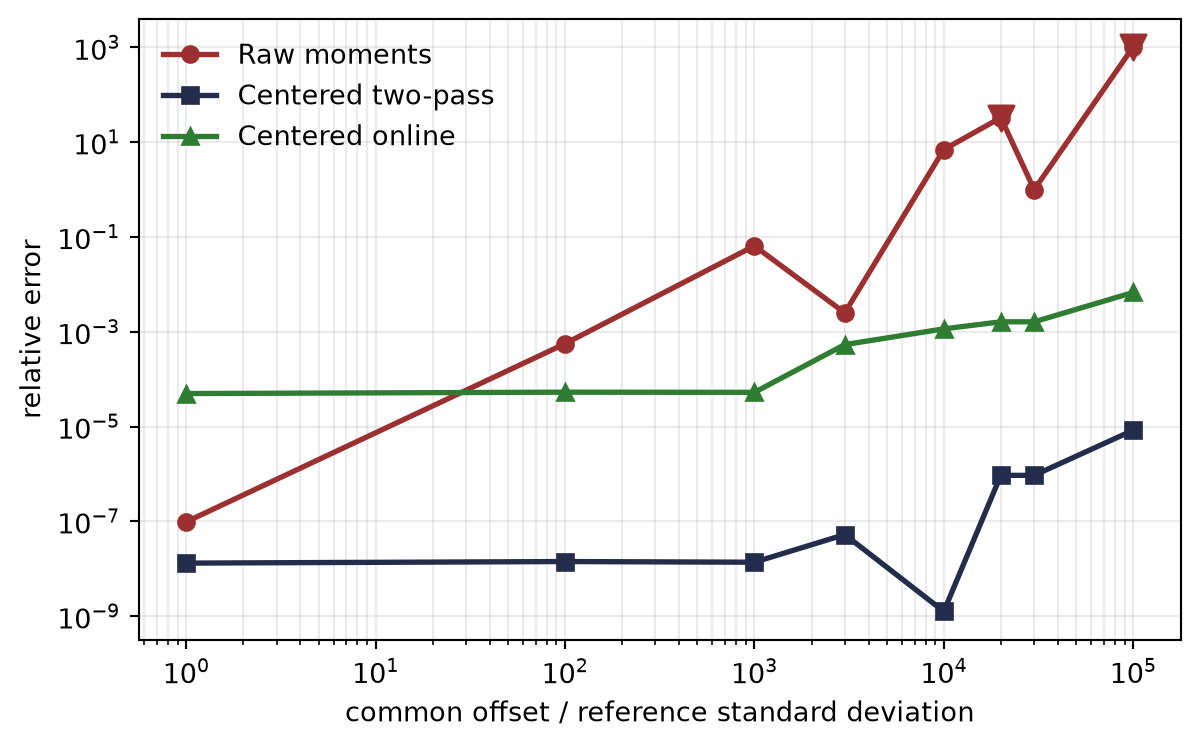
Use the same deviations at every offset. This removes a tempting alternate explanation: changes in the graph cannot be attributed to a new random sample.

Hold one random deviation vector fixed.
Add offsets without changing the exact centered variance.
Evaluate all methods on the same represented inputs.
Plot relative error and mark impossible negative results.

# [1]
offset_rng = np.random.default_rng(6210)
deviations = offset_rng.normal(size=200_000)

# [2]
offsets = np.array([0, 100, 1_000, 3_000, 10_000, 20_000, 30_000, 100_000])

# [3]
records = []
for offset in offsets:
    represented = (offset + deviations).astype(np.float32)
    result = comparison_audit(represented, dtype=np.float32)
    scale = result["reference"]["population_variance"] ** 0.5
    records.append(
        {
            "ratio": max(float(offset / scale), 1.0),
            "naive": result["naive"]["relative_error"],
            "two_pass": result["two_pass"]["relative_error"],
            "welford": result["welford"]["relative_error"],
            "naive_negative": result["naive"]["population_variance"] < 0,
        }
    )

# [4]
fig, ax = plt.subplots(figsize=(7.0, 4.2))
styles = {
    "naive": ("Raw moments", "#9C2F2F", "o"),
    "two_pass": ("Centered two-pass", "#232D4B", "s"),
    "welford": ("Centered online", "#2E7D32", "^"),
}
for key, (label, color, marker) in styles.items():
    ax.plot(
        [row["ratio"] for row in records],
        [max(row[key], 1e-9) for row in records],
        label=label,
        color=color,
        marker=marker,
        linewidth=2,
    )
for row in records:
    if row["naive_negative"]:
        ax.scatter(
            row["ratio"],
            max(row["naive"], 1e-9),
            color="#9C2F2F",
            marker="v",
            s=90,
            zorder=4,
        )
ax.set(xscale="log", yscale="log")
ax.set_xlabel("common offset / reference standard deviation")
ax.set_ylabel("relative error")
ax.grid(True, which="both", alpha=0.25)
ax.legend(frameon=False)
plt.show()

Log-log plot of relative variance error against offset-to-standard-deviation ratio. The raw-moment curve rises sharply and includes downward triangles for negative estimates, while two-pass and Welford curves stay much lower. — Figure 2.1: The raw-moment formula degrades as a common offset grows, although exact variance is translation invariant. Downward triangles mark negative estimates. Centered methods avoid the dominant cancellation, but the figure does not claim that they eliminate all rounding or input-quantization error.

The relevant observation is not that one curve has a particular shape. It is that a transformation which preserves exact variance changes the raw-moment answer dramatically. The experiment has isolated sensitivity to translation.

2.2 Diagnose the subtraction

Write each observation as

\[ x_i=\mu+\varepsilon_i, \qquad \frac{1}{n}\sum_i\varepsilon_i=0, \qquad \frac{1}{n}\sum_i\varepsilon_i^2=\sigma^2. \]

Then

\[ \frac{1}{n}\sum_i x_i^2=\mu^2+\sigma^2, \qquad \left(\frac{1}{n}\sum_i x_i\right)^2=\mu^2. \]

The raw-moment formula asks floating-point arithmetic to construct two values on the scale of \(\mu^2\), then subtract them to recover one on the scale of \(\sigma^2\).

Suppose, as a diagnostic model calculation, that the two large terms acquire absolute errors of order \(u\mu^2\), where \(u\) is the unit roundoff. The absolute error in their difference is then also on that scale. Relative to the desired variance, the amplification is approximately

\[ \frac{u\mu^2}{\sigma^2} = u\left(\frac{\mu}{\sigma}\right)^2. \tag{2.3}\]

This is not a complete forward-error bound for a particular summation kernel. It deliberately suppresses the number of additions, reduction order, compensation, and intermediate precision. It does explain the observed control: translating the data leaves exact variance alone while increasing the scale of the two terms that must cancel.

Named wrong answer: ‘FP32 cannot represent the noise’

At the opening offset, FP32 still represents many distinct unit-scale deviations. We know because the FP64 reference is computed after the FP32 cast and remains near one. The dominant opening failure is algorithmic cancellation, not already-lost input information.

At a sufficiently larger offset, the spacing between representable FP32 values does become comparable with the deviations. That is a different failure, and no variance algorithm can recover distinctions absent from its input.

The two failures must stay separate:

Failure	Where information is lost	Can centered state repair it?
Raw-moment cancellation	During accumulation and subtraction of large moments	It avoids the dominant subtraction
Input quantization	When real values are rounded to the input dtype	No; the distinctions never reach the algorithm

The next chapter develops the precision language needed to quantify the second row. For now, this separation is enough to design the state.

2.3 Preserve the centered invariant

The desired state after \(n\) values is

\[ h_n=(n,\mu_n,M_{2,n}), \qquad M_{2,n}:=\sum_{i=1}^{n}(x_i-\mu_n)^2. \tag{2.4}\]

The final population variance is \(M_{2,n}/n\). The usual unbiased sample variance is \(M_{2,n}/(n-1)\) when \(n>1\). The state does not need to commit to either denominator while the stream is arriving.

When \(x_n\) arrives, define its deviation from the old mean:

\[ \delta_n:=x_n-\mu_{n-1}. \]

The mean update follows directly from the definition:

\[ \mu_n = \mu_{n-1}+\frac{\delta_n}{n}. \tag{2.5}\]

The centered sum of squares uses both the old and new means:

\[ M_{2,n} = M_{2,n-1} +(x_n-\mu_{n-1})(x_n-\mu_n). \tag{2.6}\]

Theorem 2.1 (Centered-state invariant) Assume the state after \(n-1\) values satisfies

\[ M_{2,n-1}=\sum_{i=1}^{n-1}(x_i-\mu_{n-1})^2. \]

Together, the mean update and the centered-sum update above produce

\[ M_{2,n}=\sum_{i=1}^{n}(x_i-\mu_n)^2 \]

in exact arithmetic.

Proof

Let \(\delta=\delta_n\). The mean moves by \(\delta/n\), so for each old observation,

\[ x_i-\mu_n=(x_i-\mu_{n-1})-\frac{\delta}{n}. \]

Expand the contribution from the first \(n-1\) values:

\[ \begin{aligned} \sum_{i=1}^{n-1}(x_i-\mu_n)^2 &= \sum_{i=1}^{n-1}(x_i-\mu_{n-1})^2 \\ &\quad -\frac{2\delta}{n} \sum_{i=1}^{n-1}(x_i-\mu_{n-1}) +(n-1)\frac{\delta^2}{n^2}. \end{aligned} \]

The middle term vanishes because deviations from \(\mu_{n-1}\) sum to zero. The new observation contributes

\[ (x_n-\mu_n)^2 = \left(\delta-\frac{\delta}{n}\right)^2 = \left(\frac{n-1}{n}\delta\right)^2. \]

Adding the old and new contributions gives

\[ \begin{aligned} M_{2,n} &=M_{2,n-1} +(n-1)\frac{\delta^2}{n^2} +(n-1)^2\frac{\delta^2}{n^2}\\ &=M_{2,n-1}+\frac{n-1}{n}\delta^2. \end{aligned} \]

Finally,

\[ (x_n-\mu_{n-1})(x_n-\mu_n) = \delta\left(\frac{n-1}{n}\delta\right), \]

which is exactly the increment added by the centered-sum update. \(\square\)

The proof does more than validate a formula. It identifies the invariant the state represents after every prefix. That invariant lets us test the kernel on any prefix and gives us the object that partial computations must preserve.

The mechanism in code

Initialize the empty centered state.
Update the mean with the deviation from the old mean.
Update the centered sum using deviations from both means.
Check the kernel against the pinned harness and a direct calculation.

def welford_kernel(stream, dtype=np.float64):
    scalar = np.dtype(dtype).type
    count, mean, m2 = 0, scalar(0), scalar(0)  # [1]
    for value in np.asarray(stream, dtype=dtype):
        count += 1
        delta = scalar(value - mean)
        mean = scalar(mean + delta / scalar(count))  # [2]
        delta_after = scalar(value - mean)
        m2 = scalar(m2 + delta * delta_after)  # [3]
    return count, float(mean), float(m2)


small = np.array([4.0, 7.0, 13.0, 16.0, 20.0], dtype=np.float64)
kernel_state = welford_kernel(small)
harness_state = stable_online_moments(small, dtype=np.float64)
direct_m2 = float(np.sum((small - small.mean()) ** 2))

assert kernel_state == (
    harness_state.count,
    harness_state.mean,
    harness_state.m2,
)
assert np.isclose(kernel_state[2], direct_m2)  # [4]
print(
    f"count={kernel_state[0]}, mean={kernel_state[1]:.1f}, "
    f"M2={kernel_state[2]:.1f}, variance={kernel_state[2] / kernel_state[0]:.1f}"
)

count=5, mean=12.0, M2=170.0, variance=34.0

The update remains a floating-point recurrence. Centering removes the particular subtraction diagnosed by Equation 2.3; it does not make every update exact. “Stable” always needs an object and a failure mode. Here it means that the algorithm avoids forming raw moments on the scale of \(\mu^2\) merely to recover a centered quantity on the scale of \(\sigma^2\).

2.4 One state must also combine

Sequential state solves the one-pass problem for one stream. It does not yet solve the execution problem for many blocks. If block \(A\) and block \(B\) are processed independently, each produces a valid state:

\[ h_A=(n_A,\mu_A,M_{2,A}), \qquad h_B=(n_B,\mu_B,M_{2,B}). \]

Adding \(M_{2,A}\) and \(M_{2,B}\) is wrong whenever the block means differ. The smallest counterexample is:

\[ A=\{0,0\}, \qquad B=\{10,10\}. \]

Both within-block variances are zero. The union has mean five and population variance 25. The missing quantity is variation between the block means.

Let

\[ \delta:=\mu_B-\mu_A, \qquad n:=n_A+n_B. \]

The combined mean is

\[ \mu_{A\cup B} = \mu_A+\delta\frac{n_B}{n}. \tag{2.7}\]

The centered sum combines as

\[ M_{2,A\cup B} = M_{2,A}+M_{2,B} +\delta^2\frac{n_A n_B}{n}. \tag{2.8}\]

Theorem 2.2 (Pairwise centered-state merge) If \(h_A\) and \(h_B\) satisfy the centered-state invariant on disjoint collections \(A\) and \(B\), then Equation 2.7 and Equation 2.8 satisfy it on \(A\cup B\).

Proof

Recenter block \(A\) around the combined mean:

\[ \begin{aligned} \sum_{i\in A}(x_i-\mu_{A\cup B})^2 &= \sum_{i\in A} \left[(x_i-\mu_A)+(\mu_A-\mu_{A\cup B})\right]^2\\ &= M_{2,A}+n_A(\mu_A-\mu_{A\cup B})^2. \end{aligned} \]

The cross term vanishes because deviations from \(\mu_A\) sum to zero. The same argument for \(B\) gives

\[ M_{2,B}+n_B(\mu_B-\mu_{A\cup B})^2. \]

From Equation 2.7,

\[ \mu_A-\mu_{A\cup B}=-\delta\frac{n_B}{n}, \qquad \mu_B-\mu_{A\cup B}=\delta\frac{n_A}{n}. \]

The two recentering costs therefore sum to

\[ \delta^2 \left( \frac{n_A n_B^2}{n^2} +\frac{n_B n_A^2}{n^2} \right) = \delta^2\frac{n_A n_B}{n}. \]

That is exactly the correction in Equation 2.8. \(\square\)

The correction measures how much centered energy appears when two local origins are replaced by one global origin.

Build one centered state per block.
Merge the states with the between-block correction.
Compare the merged result with the direct union.
Reject the tempting sum of within-block centered sums.

# [1]
left = stable_online_moments([0.0, 0.0], dtype=np.float64)
right = stable_online_moments([10.0, 10.0], dtype=np.float64)

# [2]
combined = merge_moments(left, right)

# [3]
direct = np.var(np.array([0.0, 0.0, 10.0, 10.0]), dtype=np.float64)
assert np.isclose(combined.population_variance, direct)

# [4]
without_correction = (left.m2 + right.m2) / combined.count
assert without_correction == 0.0
print(
    f"within-only={without_correction:.1f}, "
    f"with correction={combined.population_variance:.1f}"
)

within-only=0.0, with correction=25.0

Associative in which arithmetic?

In exact arithmetic, the merge operation is associative on valid states. A state represents the count, mean, and centered sum of squares of one underlying multiset. Both

\[ (h_A\oplus h_B)\oplus h_C \quad\text{and}\quad h_A\oplus(h_B\oplus h_C) \]

represent the same union, whose three exact statistics are unique.

That statement gives us a parallel reduction tree. It does not say that floating-point parenthesizations are bitwise identical. Each merge rounds, so the tree becomes part of the numerical algorithm.

Form the same FP32 block states once.
Merge them left-to-right, right-to-left, and in a balanced tree.
Retain a sequential state and same-input FP64 reference as controls.
Report the spread without declaring one order universally best.

# [1]
order_rng = np.random.default_rng(6211)
order_values = (20_000.0 + order_rng.normal(size=131_072)).astype(np.float32)
blocks = [
    stable_online_moments(block, dtype=np.float32)
    for block in np.array_split(order_values, 128)
]

def left_fold(states):
    state = states[0]
    for next_state in states[1:]:
        state = merge_moments(state, next_state)
    return state


def balanced_fold(states):
    level = list(states)
    while len(level) > 1:
        level = [
            merge_moments(level[index], level[index + 1])
            if index + 1 < len(level)
            else level[index]
            for index in range(0, len(level), 2)
        ]
    return level[0]

# [2]
orders = {
    "left": left_fold(blocks),
    "right": left_fold(list(reversed(blocks))),
    "balanced": balanced_fold(blocks),
}

# [3]
orders["sequential"] = stable_online_moments(order_values, dtype=np.float32)
order_reference = float(np.var(order_values.astype(np.float64)))

# [4]
for name, state in orders.items():
    print(
        f"{name:>10}: variance={state.population_variance:.9f}, "
        f"error={abs(state.population_variance - order_reference):.3e}"
    )
print(f"{'reference':>10}: variance={order_reference:.9f}")

      left: variance=0.998615682, error=1.937e-04
     right: variance=0.998613298, error=1.913e-04
  balanced: variance=0.998613000, error=1.910e-04
sequential: variance=1.000126481, error=1.704e-03
 reference: variance=0.998421996

The three merge trees differ in their final bits, as expected. The balanced tree is not promoted here as a universal accuracy theorem: data order, partial-state quality, accumulator width, and the implementation of the combine all matter. The supported claim is narrower. A mathematical combine law creates parallel structure; floating-point execution still requires a reduction-order audit.

2.5 Choosing the state is choosing the algorithm

The original question was not “which variance formula should a library use?” The useful question is “what constraints does this execution have?”

Constraint	Honest baseline	Principal cost or boundary
Data can be revisited	Centered two-pass variance	Reads the input at least twice
True one-pass stream	Sequential centered state	Dependency depth grows with stream length
Independent blocks	Centered partial states plus pairwise merge	Floating-point tree order affects final bits
Input distinctions already lost	Wider storage or an upstream scaling change	No downstream state can reconstruct missing values

The raw-moment formula remains an algebraic identity. Its failure does not make the identity false. It makes the evaluation path unsuitable in the observed regime.

The same centered state later appears inside batch-coordinate normalization: its running statistics are mergeable estimates whose axes, denominator, update rule, and accumulator precision must be declared explicitly.

Field note: what a trace can and cannot tell you

A negative variance strongly implicates numerical execution because exact variance is nonnegative. A merely inaccurate positive variance is less diagnostic. It can come from cancellation, input quantization, accumulation order, a mismatched denominator, or a changing target. Record the state, dtype, axes, denominator, and same-input reference before assigning a cause.

Check yourself

You have two blocks whose internal variances are both zero, but whose means differ. Why is adding the two \(M_2\) values wrong? Which single term repairs the result, and what does that term measure?

2.6 Okay, so —

Inherited: A formula has a data-movement schedule; rereading a tensor is an algorithmic decision.
Changed: Variance is no longer just a definition. It is a state-design problem constrained by passes, rounding, and parallel structure.
Instrumented: The harness now records the execution contract, compares methods on the same represented inputs, maintains centered moments, and merges partial states.
Established: The centered online recurrence and the pairwise correction preserve \(M_2\) in exact arithmetic. The seeded FP32 witness establishes that the raw-moment evaluation can return an impossible negative result.
Unresolved: Which precision contract separates values lost at storage from errors introduced by a non-associative reduction?

2.7 Sources and further reading

The corrected online update traces to Welford’s short note (Welford 1962). Chan, Golub, and LeVeque compare variance algorithms, analyze roundoff, and develop pairwise computation (Chan et al. 1983).

Hennig, Pförtner, and Weiland frame limited computation as limited information (Hennig et al. 2026). Hennig makes one version exact for iterative linear solvers under a declared Gaussian model (Hennig 2015). That work motivates Exercise 7; it does not make the centered-moment recurrence a Bayesian update.

For floating-point format anatomy, mixed-precision roles, and introductory rounding examples, see the sibling volume’s precision and hardware appendix. This chapter instead owns the centered invariant, merge law, and same-input diagnostic.

Reading order. Start with Welford (1962) for the recurrence and Chan et al. (1983) for the stability and merge analysis; read Hennig (2015) only after the chapter’s state-versus-belief boundary is clear.

2.8 Exercises

(Pencil.) The invariant from another direction. Starting from \(M_{2,n}=\sum_{i=1}^{n}x_i^2-n\mu_n^2\), derive the centered-sum update stated in this chapter. Mark the step that is safe as an exact identity but would reintroduce the raw-moment hazard if used as the implementation.
(Pencil.) Population versus sample. Prove that the same state \((n,\mu_n,M_{2,n})\) can produce either the population variance or the usual unbiased sample variance. Explain why changing the final denominator cannot repair catastrophic cancellation already present in \(M_{2,n}\).
(Code.) Crash map. Hold one represented deviation vector fixed and sweep both offset and accumulator dtype. Report the first offset at which the raw-moment estimate becomes negative and the first at which the centered methods exceed one percent relative error. Keep the FP64 reference on the same represented inputs.
(Code.) Profile: one pass versus two. On a laptop CPU, compare bytes implied by one-pass and two-pass schedules for a contiguous FP32 array. Time the implementations only after stating warmup, sample count, and estimator. Do not interpret CPU timing as accelerator performance.
(Audit.) The clipped repair. A code review proposes variance = max(raw_variance, 0). Predict which visible symptom this removes, then design a test showing what error it conceals. State the strongest claim the clipped result can support.
(Audit.) Merge contract. An implementation all-reduces only \((n,\mu,M_2)\) by componentwise sum. Use two constant blocks to identify the defect. Write the missing correction and explain why the tempting componentwise answer is wrong.
(Audit.) Paper audit: state versus belief. Complete the Mathematical object, Evidence culture and interface, Estimator and comparison contract, Assumption stress test, and Transfer verdict fields for Hennig’s Gaussian linear-solver construction (Hennig 2015). Compare its state \((\vect{\mu}_i,\matr{\Sigma}_i)\) with Welford’s \((n,\mu_n,M_{2,n})\): record the target, observation, prior, rank-one update, stopping output, and uncertainty claim. Identify the shared state-machine pattern, then explain why Welford is not Bayesian conditioning without an additional probability model.