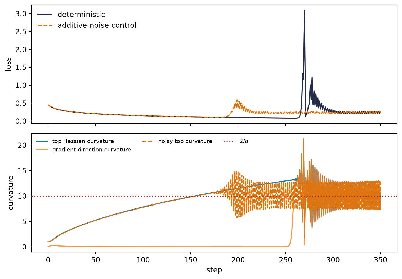
starting from the origin. The top Hessian eigenvalue begins at one, far below the fixed-quadratic boundary \(2/\alpha=10\). At step 155 it first crosses ten. Across 350 steps the loss increases 52 times, while the trajectory remains in a bounded, structured oscillatory regime. A stability test performed only at initialization gives the correct answer to the wrong time-indexed question.
ImportantPrediction
If the top curvature crosses \(2/\alpha\), must a nonlinear training run diverge immediately? Choose between immediate divergence, a diagnostic event whose consequence must be measured, and no information at all. Which control would distinguish your choice from the other two?
16.1 The fixed control
Theorem 16.1 (Exact stability of one quadratic mode) For \(f(z)=\lambda z^2/2\) with \(\lambda>0\), gradient descent gives \(z_{k+1}=(1-\alpha\lambda)z_k\). The iterates converge to zero exactly when
\[
0<\alpha\lambda<2.
\tag{16.2}\]
Proof
The recurrence converges precisely when its scalar multiplier has magnitude less than one: \(|1-\alpha\lambda|<1\). At \(\alpha\lambda>1\), signs alternate; at two, the mode has a perfect two-cycle; beyond two, its magnitude grows.
For a positive-definite quadratic, apply the result to every eigenmode. This is C04’s fixed spectral boundary. It is the indispensable control—not a license to substitute a local Hessian eigenvalue into a global conclusion.
We record both \(\lambda_{\max}(\nabla^2f)\) and gradient-direction curvature \(\vect g^{\mathsf T}\nabla^2f\vect g/\|\vect g\|^2\). The first asks for the worst local direction; the second asks what curvature the current update actually sees. C12 already warned that the matrix itself must be named.
Load the chapter-pinned stability instruments.
Run matched deterministic and additive-noise trajectories.
Record loss, top curvature, and gradient-direction curvature each step.
Mark the fixed-quadratic threshold and first crossing.
Verify both committed crossing and nonmonotonicity claims.
Figure 16.1: A trajectory can begin below the quadratic stability edge and later move the local top curvature across it. A small additive-noise contrast preserves the crossing but shifts its timing and loss increments; neither trace turns a local quadratic threshold into a global divergence theorem.
Claims c16-moving-boundary-001, c16-stochastic-contrast-001 · seed: deterministic primary trajectory; registered stochastic control · dtype: FP64 · device: CPU · estimator: top and directional curvature along the realized path · artifact
This is a laptop-exact demonstration: minutes are not needed, no GPU is required, and every point is regenerated on a CPU. It establishes the logical possibility of a moving boundary. The additive-noise trace crosses at step 156 rather than 155 and contains 91 loss increases rather than 52. It shows that the crossing story survives this small perturbation while its timing and nonmonotonicity do not. Neither trace claims that a two-parameter valley reproduces mini-batch training or every feature of a large run.
16.3 One boundary, two diagnostic objects
The exact quadratic and the nonlinear trajectory should be read in one panel, not as consecutive stories:
Diagnostic field
Fixed quadratic control
Moving nonlinear trajectory
What transfers
state
one eigenmode \(z_k\)
parameter vector \(\vect w_k\)
compare the update with curvature at the same time index
curvature
constant scalar \(\lambda\)
\(\lambda_{\max}(\matr H_k)\) and gradient-direction curvature
\(2/\alpha\) remains a reference scale
prediction
exact convergence iff \(0<\alpha\lambda<2\)
crossing is an event to investigate
sign alternation and local aggressiveness remain useful clues
history
one fixed multiplier
rotating directions and changing Hessian
the trajectory must be recorded
conclusion
necessary and sufficient for this mode
no universal divergence verdict
the quadratic is a control, not a theorem about the full run
The matched panel slows the transfer at the point where it is easiest to overreach. “Above two” is an exact statement only in the left column.
16.4 Local Taylor information is historical
For one update \(\vect w^+=\vect w-\alpha\vect g\), Taylor’s theorem along the segment gives
for some \(\tau\in(0,1)\). The relevant curvature can lie between endpoints, and a top eigenvector can be nearly orthogonal to the step. Consequently a credible edge-of-stability panel reports at least step size, top curvature, directional curvature, loss increments, estimator/batch regime, and the curvature operator used.
16.5 From witness to empirical phenomenon
Large full-batch training runs have been observed to approach and operate near the classical threshold, with progressive sharpening and nonmonotone loss (Cohen et al. 2021). A useful one-line contrast is: classical optimization adapts the step to a curvature bound; deep compositional structures can move their local curvature toward the chosen step. This is an empirical organizing statement, not a universal convergence theorem.
The “staircase” behavior analyzed in later edge-of-stability work belongs in the paper-audit branch: students should identify its model, timescale, and measured curvature before treating it as the same phenomenon. The trunk keeps the fixed quadratic, the moving witness, and the measurement contract.
WarningNamed wrong answer: above two means divergent
Above two means divergent for a fixed positive quadratic eigenmode. A local nonlinear Hessian can rotate and change after the step; crossing is a diagnostic event whose consequences must be measured.
16.6 Numerical stability returns
Near an oscillatory boundary, small arithmetic changes can alter which side of a narrow basin an update reaches. That does not make every loss spike a precision failure. It means curvature, reduction order, storage/accumulation format, and replay determinism belong in one incident report. The four threads have converged on a common diagnostic discipline.
16.7 Check yourself
For a fixed mode with \(\lambda=12\) and \(\alpha=0.2\), what is the multiplier and what does it imply? For a nonlinear objective whose local top eigenvalue is 12 at one point, which additional measurements would be needed before predicting the next several iterates?
16.8 Okay, so —
Inherited: C04 supplies the exact fixed-quadratic boundary and C12 supplies operator-specific curvature probes.
Changed: stability is treated as a trajectory diagnosis, not an initialization certificate.
Instrumented: matched deterministic and additive-noise traces track top and directional curvature beside loss.
Established: a reproducible nonlinear path can cross \(2/\alpha\) after beginning below it.
Unresolved: Which norm should shape a matrix-valued update when scalar curvature says only where one step struggles?
16.9 Sources and further reading
The edge-of-stability phenomenon and progressive sharpening measurements are documented by Cohen et al. (2021). The fixed control is elementary spectral gradient descent.
Reading order. Start with Cohen et al. (2021) for the measurements, then return to the fixed quadratic theorem in C04 before transferring the observed threshold to a moving nonlinear trajectory.
16.10 Exercises
(Pencil.) Derive the momentum stability polynomial for one positive quadratic mode, explicitly limiting the conclusion to that control.
(Code.) Sweep step size in Equation 16.1 and produce a phase diagram of first threshold crossing, loss increases, and boundedness.
(Pencil.) Use Equation 16.4 to give a sufficient one-step descent condition in terms of the maximum directional curvature along the update segment. Explain why endpoint curvature alone is weaker.
(Code.) Repeat the paired contrast over noise scales and seeds. Report crossing probability, crossing time, loss-increase count, and boundedness; keep the deterministic trace as a registered control.
(Audit.) Paper audit: Complete the Mathematical object, Resolution of the theory, Dynamic regime, Evidence culture and interface, Discriminating control, and Transfer verdict fields of the Paper Autopsy Protocol for an edge-of-stability result. Record curvature operator, eigenvalue estimator, batch regime, sampling frequency, threshold convention, and whether crossing predicts or merely accompanies the reported behavior.
Cohen, Jeremy M., Simran Kaur, Yuanzhi Li, J. Zico Kolter, and Ameet Talwalkar. 2021. “Gradient Descent on Neural Networks Typically Occurs at the Edge of Stability.”International Conference on Learning Representations. https://openreview.net/forum?id=jh-rTtvkGeM.