Let \(Z\sim\mathcal{N}(0,1)\). C05 puts \(Z\) safely inside a global quadratic MGF envelope. Now perform one of the most ordinary operations in computation:
\[
X=Z^2-1.
\]
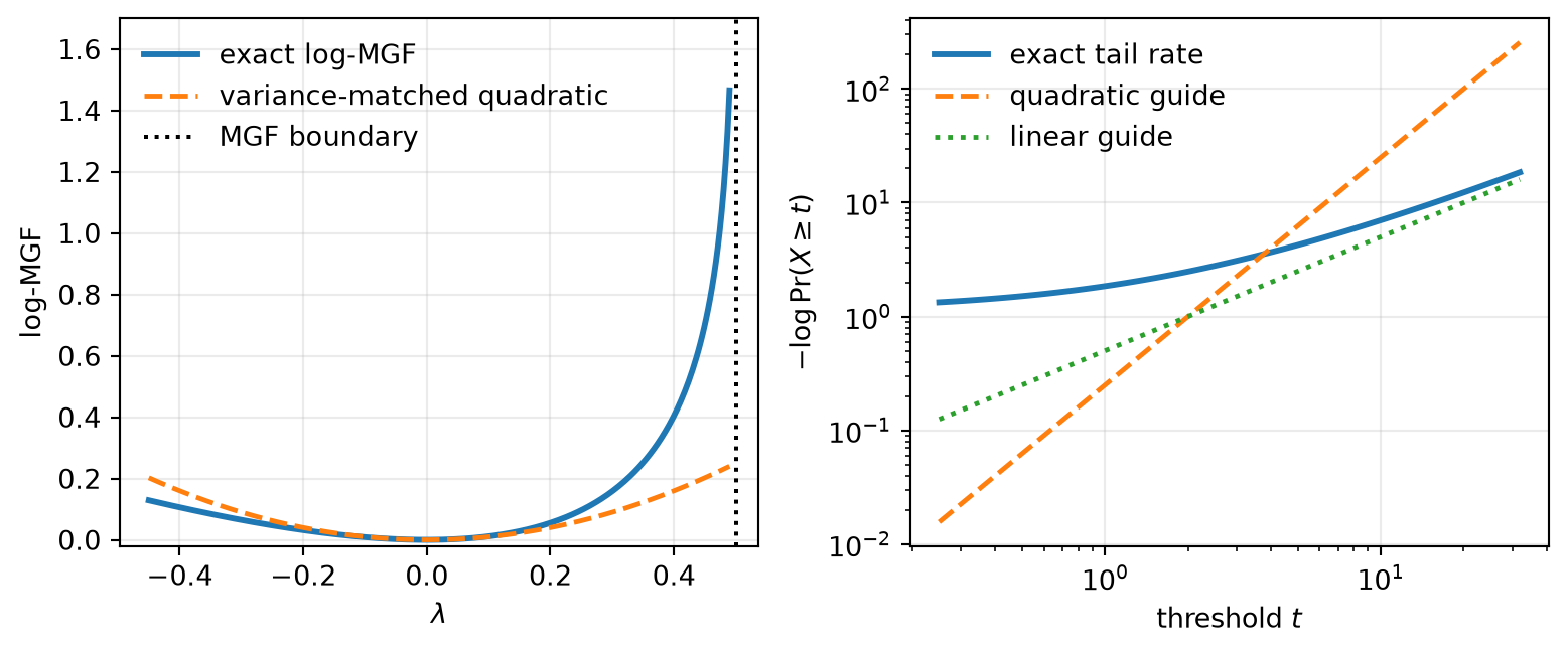
The centering makes \(\E X=0\), and \(\var(X)=2\). Neither fact saves the old tail contract. On the declared threshold grid, the exact upper tail at \(t=4\) is about \(0.02535\), already larger than the variance-matched quadratic candidate \(e^{-t^2/4}\approx0.01832\). At \(t=8\), the gap is no longer close.
ImportantPrediction
Which diagnosis survives a stronger test?
The variance proxy merely needs a slightly larger constant.
Centering should eventually restore a global quadratic envelope.
Squaring changed the domain on which the MGF exists.
Choose before inspecting the generating function. Then predict which step of C05’s Chernoff optimization will become constrained.
6.1 Inspect the domain, not only the variance
For this distribution the MGF is available in closed form. The opening study places its log beside a variance-matched quadratic candidate and then compares the exact upper-tail rate with quadratic and linear guides. A guide is not a probability bound; its job is to expose the shape that eventually becomes impossible.
Load the chapter-pinned tail instruments.
Evaluate the exact log-MGF below its finite boundary.
Evaluate exact upper tails on a declared threshold grid.
Locate the first failure of a variance-matched quadratic candidate.
Figure 6.1: A square breaks the global quadratic contract. At left, the exact log-MGF of the centered Gaussian square rises toward a singularity at one half, so no finite parabola can dominate it on all positive parameters. At right, the exact upper-tail rate bends toward linear growth while the variance-matched quadratic candidate becomes far too optimistic. The guides diagnose shape; only the exact MGF domain proves non-sub-Gaussianity.
At \(\lambda\ge1/2\), the integrand no longer decays at infinity. Centering removes the linear term near the origin; it cannot reopen the MGF after the quadratic transform has closed it.
6.2 The square keeps an exponential contract
The safe zone did not disappear. It became smaller. Define
A random variable with finite \(\psi_1\) norm is called sub-exponential. The name describes an exponential tail class; it does not mean that the random variable itself is an exponential distribution.
Theorem 6.1 (Squares and products remain sub-exponential) If \(X\) is sub-Gaussian, then
Let \(a=\norm{X}_{\psi_2}\). The defining condition \(\E e^{X^2/a^2}\le2\) is exactly the condition that \(\norm{X^2}_{\psi_1}\le a^2\). Taking the infimum in both definitions gives equality in Equation 6.3.
so \(\E X^2\le a^2\log2\). A constant \(c\) has \(\psi_1\) norm \(|c|/\log2\). The triangle inequality for the Orlicz norm therefore yields Equation 6.4.
For the product, put \(a=\norm{X}_{\psi_2}\) and \(b=\norm{Y}_{\psi_2}\). The elementary inequality
Squaring destroys the global quadratic MGF envelope. It leaves an exponential-moment contract, which is strong enough for useful concentration but changes the deviation rate and the diagnostic scale.
6.3 A local parabola creates two regimes
A centered sub-exponential variable still looks quadratic near \(\lambda=0\). The difference from C05 is the quantifier:
Tail contract
Quadratic log-MGF bound
Chernoff optimizer
sub-Gaussian
every real \(\lambda\)
unconstrained
sub-exponential
only \(|\lambda|\le c/K\)
constrained
no positive MGF
no interval to the right of zero
unavailable
The sub-exponential equivalence theorem makes the middle row precise: for a centered \(X\), there are universal constants \(c_0,C_0>0\) such that
As in C05, tail, moment, exponential-moment, and local-MGF characterizations are equivalent up to universal constants. The new fact is that the admissible interval is finite.
Theorem 6.2 (Bernstein’s two-regime inequality) Let \(X_1,\ldots,X_n\) be independent, centered, sub-exponential random variables. Write
If the first argument is smaller, substitution into Equation 6.8 gives an exponent at most \(-c_1t^2/V\). If the second is smaller, the inequality defining that case lets the quadratic term absorb at most a fixed fraction of \(\lambda t\), leaving an exponent at most \(-c_2t/B\). Apply the same argument to \(-X_i\), add the two tails, and take \(c=\min(c_1,c_2)\). \(\square\)
The transition occurs near \(t=V/B\). If all \(\psi_1\) scales are comparable to \(K\), then \(V/B\asymp nK\). Averaging has not failed: increasing \(n\) extends the quadratic regime. What changes is the far tail, where the desired Chernoff parameter would lie outside the MGF’s admissible interval.
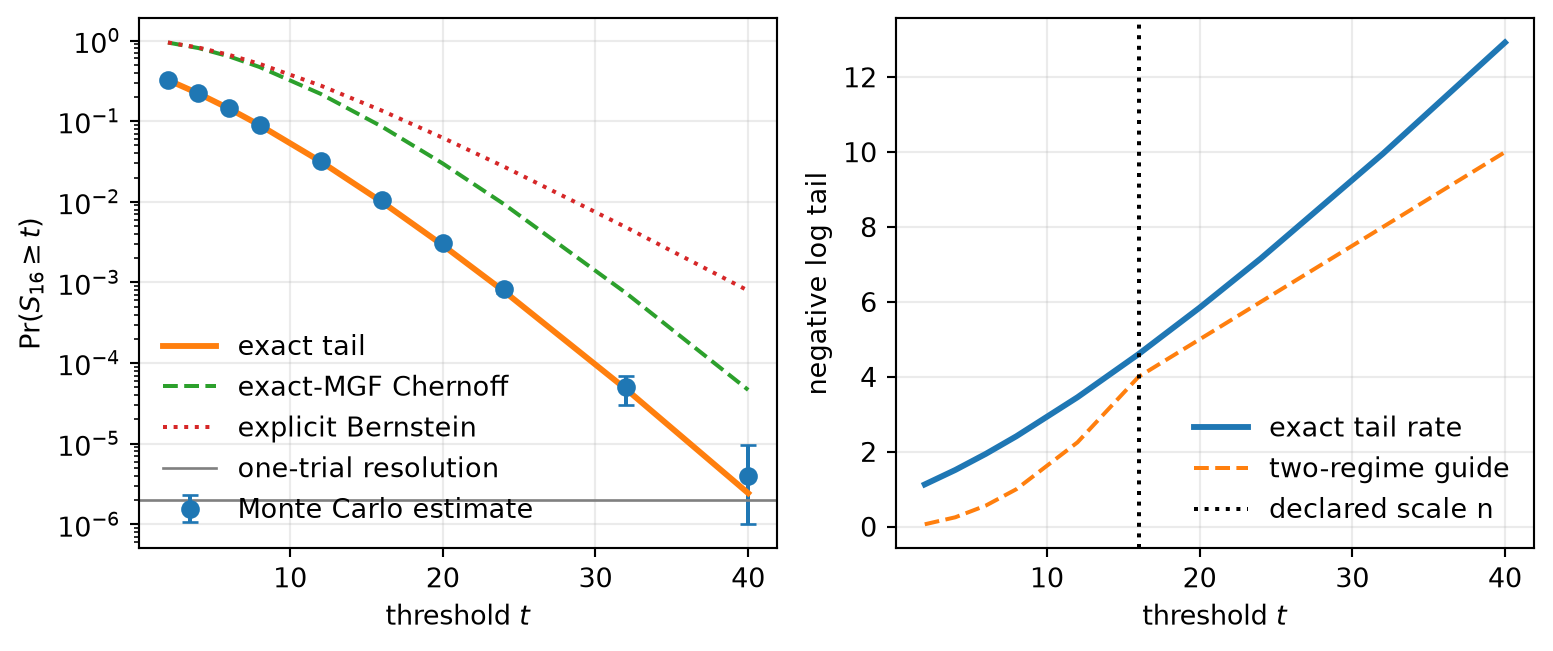
Because the degrees of freedom are even, its exact upper tail is a finite series. That exact curve is the control. Monte Carlo is shown only where its 500,000-trial denominator has resolution.
Figure 6.2: A centered chi-square sum retains two distinct deviation scales. At left, 500,000 seeded trials track the exact upper tail until only a few exceedances remain; exact probabilities continue beyond simulation resolution. Both analytic controls remain upper bounds. At right, the exact negative log tail bends from a quadratic toward a linear rate around the declared scale n equals 16. The experiment validates this distribution-specific witness, not every sub-exponential sum.
At \(t=40\), the simulation sees only two exceedances. The exact tail is about \(2.43\times10^{-6}\), while the estimate is \(4.00\times10^{-6}\) with standard error about \(2.83\times10^{-6}\). Reporting only the empirical curve would make the most interesting region the least trustworthy one. The exact control prevents a plotting artifact from becoming a tail claim.
6.5 When no positive MGF exists
Sub-exponential is not a synonym for every distribution heavier than a Gaussian. It is still an exponential-moment class. A Pareto variable with power-law survival has no finite positive MGF, so neither C05’s global optimization nor Bernstein’s local optimization begins.
One possible intervention maps a scalar \(x\) to a bounded interval:
This operation is conventionally called clipping. It creates a new random variable. The distinction between new tail behavior and the old target is the whole contract.
Theorem 6.3 (Concentration and bias after clipping) Let \(X\) be integrable and \(C>0\). Then
\(T_C(X)\) lies in an interval of length \(2C\). Hoeffding’s lemma applied after centering gives Equation 6.12. Equation Equation 6.13 is the difference between the expectation of the transformed estimator and the original target. Boundedness imposes no reason for that difference to vanish. \(\square\)
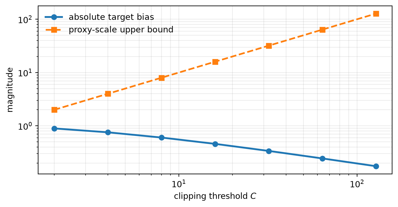
The tradeoff is exact for a simple control. Let \(Y\) have Pareto shape \(3/2\) and scale \(1\), so \(\E Y=3\) but \(\var(Y)=\infty\), and put \(X=Y-3\). For every \(C\ge2\),
Figure 6.3: Bounding a heavy-tailed variable creates opposing costs. Increasing the clipping threshold reduces the exact mean bias of the centered Pareto control, but the worst-case sub-Gaussian proxy scale of the centered clipped variable grows with that threshold. The curves establish a model tradeoff; they do not prescribe a training threshold.
NoteField note: the guardrail must itself be computable
For vector norm clipping, the norm is usually formed from a reduction of squares. If that reduction overflows before the threshold comparison, clipping never gets a finite input. C03’s precision ledger still applies: use a declared wider accumulator or a scaled sum-of-squares kernel. A post-overflow guardrail is not a guardrail.
Field
Clipping audit
Target
the original population mean or gradient
Estimator
the mean of bounded transformed observations
Reduction
over the declared sample or mini-batch
Validity
concentrated for the transformed target; useful for the original target only with a bias argument
Boundary
threshold choice, direction distortion, state dependence, and pre-clip numerical overflow remain
Empirical reports of heavy-tailed stochastic gradients are research evidence, not a universal law. Tail-index estimates depend on the model, data, mini-batch construction, training time, and estimator (Simsekli et al. 2019). Convergence guarantees for clipped stochastic updates likewise depend on the threshold and noise assumptions (Koloskova et al. 2023). C13 will turn those dependencies into a dynamic audit.
TipCheck yourself
Suppose independent centered variables have \(\norm{X_i}_{\psi_1}\le3\) for \(i=1,\ldots,100\). Up to universal constants, identify the transition scale \(V/B\). Which Bernstein exponent controls at \(t=30\) and at \(t=3000\)? Then state why finite variance alone would not justify either answer.
6.6 Okay, so —
Inherited: C05 supplied a global quadratic MGF envelope, a \(\psi_2\) scale, and the Chernoff optimizer.
Changed: one square restricts the MGF domain and replaces one global quadratic tail regime with Bernstein’s quadratic-to-linear pair.
Instrumented: the harness now evaluates exact centered-chi-square MGFs and tails, seeded sum tails, Bernstein rates, and exact clipping bias.
Established: squares and products of sub-Gaussian variables are sub-exponential; independent centered sub-exponential sums obey a two-regime bound; bounded transforms concentrate around their own means.
Unresolved: How can a finite tail budget control an uncountable supremum without sampling directions and hoping the maximum was found?
6.7 Sources and further reading
Vershynin develops sub-exponential equivalences, the square/product lemmas, and Bernstein’s inequality (Vershynin 2026). Hoeffding’s bounded-variable lemma supplies the clipped-variable guarantee (Hoeffding 1963). Simsekli, Sagun, and Gurbuzbalaban provide a primary empirical tail-index study (Simsekli et al. 2019), while Koloskova, Hendrikx, and Stich analyze the stochastic bias and threshold dependence of gradient clipping (Koloskova et al. 2023).
For the general theory, use Vershynin (2026); this chapter’s contribution is the squared-quantity witness and the audit that clipping changes the target.
Reading order. Start with Vershynin (2026) for the square, product, and Bernstein machinery; use Simsekli et al. (2019) and Koloskova et al. (2023) to audit the heavy-tail evidence and the target changed by clipping.
6.8 Exercises
(Pencil.) The exact Orlicz scale. Derive \(\norm{Z}_{\psi_2}^2=8/3\) directly from the Gaussian integral. Then use the definitions, not a tail equivalence theorem, to obtain \(\norm{Z^2}_{\psi_1}=8/3\).
(Pencil.) Products without independence. Rework the proof of Equation 6.5 and mark the exact line where Cauchy–Schwarz replaces independence. Construct dependent \(X,Y\) for which the conclusion remains useful.
(Code.) Resolve the transition. Repeat the centered-square sum study for \(n\in\{4,16,64\}\) under one predeclared total draw budget. Plot thresholds as multiples of \(n\) and report exceedances, denominators, and binomial intervals. Separate failure to resolve a tail from evidence that its probability is zero.
(Code.) A clipping target audit. Compare symmetric clipping on a symmetric Student distribution and the skewed Pareto control. Use matched thresholds and sample counts. Predict the sign of the bias before running, then report the transformed target and the original target separately.
(Audit.) The finite-sample certificate. A report fits a straight line to a log-survival plot over two decades and declares the population sub-exponential. Name two heavier-tailed alternatives that can mimic that window, state what the plot can falsify, and design a held-out threshold audit.
(Audit.) Paper audit: a tail-index claim. Complete the Mathematical object, Dynamic regime, Estimator and comparison contract, Assumption stress test, and Transfer verdict fields for Simsekli, Sagun, and Gurbuzbalaban (Simsekli et al. 2019). Extract the random variable whose tail is modeled, the estimator used for its index, the sampling unit, and the architecture/data/training regimes tested. Identify which statements are empirical observations, which invoke an \(\alpha\)-stable model, and which would be invalid if transferred as a universal law to a new training run.
Hoeffding, Wassily. 1963. “Probability Inequalities for Sums of Bounded Random Variables.”Journal of the American Statistical Association 58 (301): 13–30. https://doi.org/10.1080/01621459.1963.10500830.
Koloskova, Anastasia, Hadrien Hendrikx, and Sebastian U. Stich. 2023. “Revisiting Gradient Clipping: Stochastic Bias and Tight Convergence Guarantees.”Proceedings of the 40th International Conference on Machine Learning, Proceedings of machine learning research, vol. 202: 17343–63. https://proceedings.mlr.press/v202/koloskova23a.html.
Simsekli, Umut, Levent Sagun, and Mert Gurbuzbalaban. 2019. “A Tail-Index Analysis of Stochastic Gradient Noise in Deep Neural Networks.”Proceedings of the 36th International Conference on Machine Learning, Proceedings of machine learning research, vol. 97: 5827–37. https://proceedings.mlr.press/v97/simsekli19a.html.
Vershynin, Roman. 2026. High-Dimensional Probability: An Introduction with Applications in Data Science. 2nd ed. Cambridge Series in Statistical and Probabilistic Mathematics. Cambridge University Press. https://www.math.uci.edu/~rvershyn/papers/HDP-book/HDP-book.html.