4  One Step, Many Clocks: Quadratic Stability and Conditioning

LG · Landscape and update geometry Geometric supporting · Dynamic primary · Algorithmic supporting

One update rule acts on the two coordinates of

\[ \loss(\vect{e}) = \frac12\vect{e}^{\mathsf T} \begin{bmatrix} 1&0\\ 0&100 \end{bmatrix} \vect{e}, \qquad \vect{e}_0= \begin{bmatrix} 1\\1 \end{bmatrix}. \tag{4.1}\]

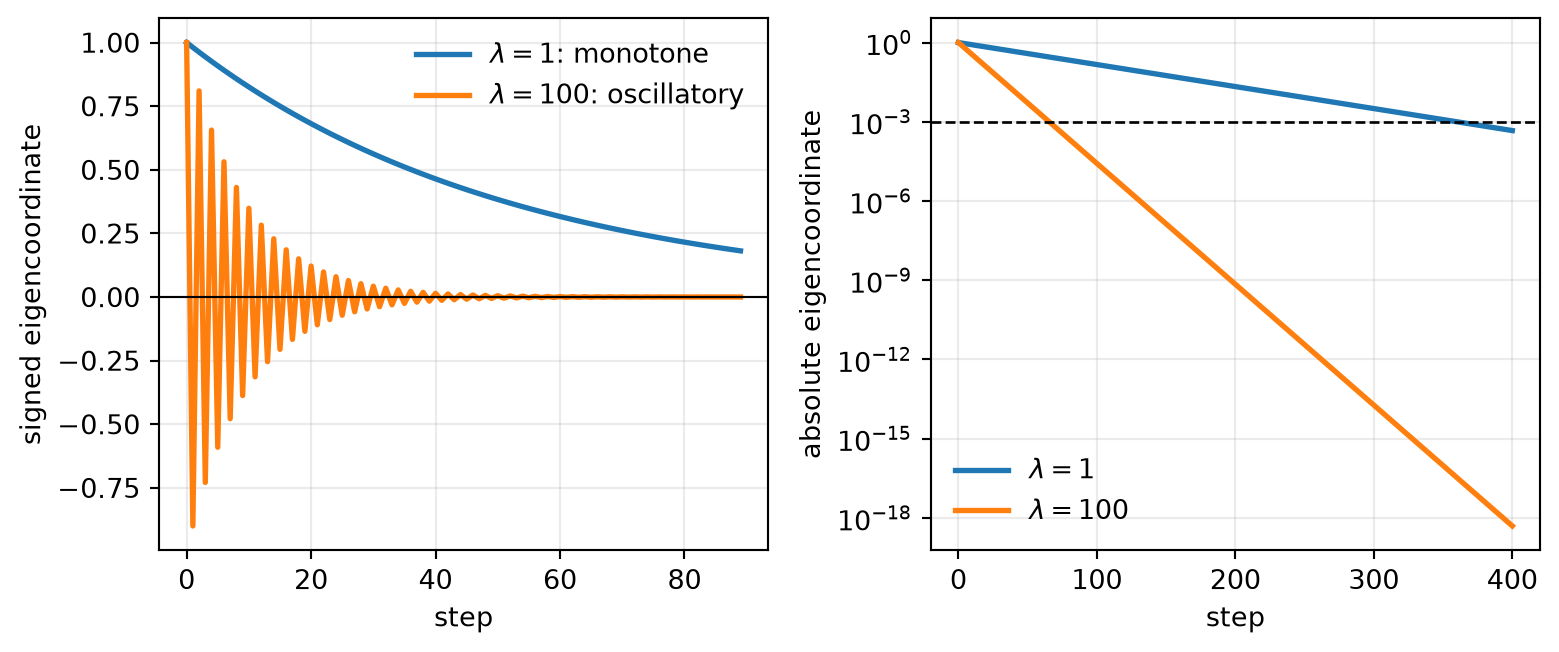
The step size is \(\alpha=0.019\). It is below the classical stability limit. The objective decreases at every step. Yet the second coordinate crosses zero on every update while the first coordinate appears almost frozen.

ImportantPrediction

Before running the recurrence, decide:

1. Which coordinate limits the largest safe step?
2. Which coordinate determines the time needed to reach a small error?
3. Can a decreasing scalar objective reveal the sign alternation?

Name the quantity you would record to distinguish the three answers.

4.1 Rotate the trace, not the story

A first optimization course supplies the update \(\vect{w}_{t+1}=\vect{w}_t-\alpha\nabla\loss(\vect{w}_t)\). The diagnostic question begins after that line: what does the update do in each direction?

The opening study uses a centered quadratic, so \(\vect{e}_t\) is both the iterate and the error from the minimizer. It verifies and activates its exact vendored harness wheel before importing the quadratic instruments.

1. Load the chapter-pinned quadratic instruments.
2. Run four hundred exact quadratic steps.
3. Rotate the iterates into Hessian eigencoordinates.
4. Assert the closed form and classify the mode factors.
5. Plot signed and absolute mode coordinates.

import matplotlib.pyplot as plt
import numpy as np

# [1]

from trainable_harness import (
    classify_mode_factors,
    quadratic_spectrum,
    quadratic_trace,
    scalar_noisy_quadratic_trials,
)

# [2]
hessian = np.diag([1.0, 100.0])
initial_error = np.array([1.0, 1.0])
step_size, steps = 0.019, 400
trace = quadratic_trace(
    hessian,
    initial_error,
    step_size=step_size,
    steps=steps,
)

# [3]
mode_coordinates = trace.mode_coordinates
eigenvalues = trace.eigenvalues

# [4]
factors, labels = classify_mode_factors(
    eigenvalues,
    step_size=step_size,
)
closed_form = factors[None, :] ** np.arange(steps + 1)[:, None]
assert np.allclose(mode_coordinates, closed_form)
assert np.all(np.diff(trace.objectives) < 0)
tolerance = 1e-3
waits = [
    int(np.ceil(np.log(tolerance) / np.log(abs(factor))))
    for factor in factors
]

# [5]
fig, axes = plt.subplots(1, 2, figsize=(8.2, 3.5))
for index, (eigenvalue, label) in enumerate(zip(eigenvalues, labels)):
    axes[0].plot(
        mode_coordinates[:90, index],
        linewidth=2,
        label=fr"$\lambda={eigenvalue:g}$: {label}",
    )
    axes[1].semilogy(
        np.abs(mode_coordinates[:, index]),
        linewidth=2,
        label=fr"$\lambda={eigenvalue:g}$",
    )
axes[0].axhline(0, color="black", linewidth=0.8)
axes[0].set(xlabel="step", ylabel="signed eigencoordinate")
axes[1].axhline(tolerance, color="black", linestyle="--", linewidth=1)
axes[1].set(xlabel="step", ylabel="absolute eigencoordinate")
for ax in axes:
    ax.grid(alpha=0.25)
    ax.legend(frameon=False)
plt.tight_layout()
plt.show()

print(f"harness={manifest['harness_ref']} wheel={manifest['wheel_sha256'][:12]}")
for eigenvalue, factor, label, wait in zip(eigenvalues, factors, labels, waits):
    print(
        f"lambda={eigenvalue:g}: factor={factor:.3f}, "
        f"{label}, steps-to-1e-3={wait}"
    )

Figure 4.1: The same scalar step creates two clocks. The flat mode stays positive and decays by 0.981 per step; the sharp mode alternates sign and decays in magnitude by 0.9. The figure establishes the exact behavior of this fixed quadratic recurrence, not the behavior of a changing training landscape.

harness=ch-04 wheel=a3478fd77e8c
lambda=1: factor=0.981, monotone, steps-to-1e-3=361
lambda=100: factor=-0.900, oscillatory, steps-to-1e-3=66

The sharp mode limits the step because its multiplier reaches magnitude one first. It does not set the stopping time here. Its magnitude falls below \(10^{-3}\) after 66 steps, whereas the flat mode waits 361 steps. The scalar objective is monotone because it squares the coordinates; it cannot show that the sharp coordinate changes sign.

4.2 The update matrix is the instrument

Let \(\matr{Q}\in\mathbb{R}^{d\times d}\) be symmetric positive definite and

\[ \loss(\vect{w}) = \frac12(\vect{w}-\vect{w}^\star)^{\mathsf T} \matr{Q} (\vect{w}-\vect{w}^\star). \]

With \(\vect{e}_t:=\vect{w}_t-\vect{w}^\star\), one gradient step becomes

\[ \vect{e}_{t+1} = (\matr{I}-\alpha\matr{Q})\vect{e}_t. \tag{4.2}\]

Theorem 4.1 (Exact quadratic mode dynamics) Write \(\matr{Q}=\matr{U}\operatorname{diag}(\lambda_1,\ldots,\lambda_d) \matr{U}^{\mathsf T}\) with \(0<\lambda_{\min}\le\lambda_k\le\lambda_{\max}\) and define \(\vect{z}_t=\matr{U}^{\mathsf T}\vect{e}_t\). Then

\[ z_{k,t} = (1-\alpha\lambda_k)^t z_{k,0}. \tag{4.3}\]

All errors converge to zero exactly when

\[ 0<\alpha<\frac{2}{\lambda_{\max}}. \tag{4.4}\]

Proof

Left-multiply Equation 4.2 by \(\matr{U}^{\mathsf T}\):

\[ \vect{z}_{t+1} = \left( \matr{I} -\alpha\operatorname{diag}(\lambda_1,\ldots,\lambda_d) \right)\vect{z}_t. \]

The recurrence is diagonal, so the \(k\)th coordinate multiplies by \(1-\alpha\lambda_k\) at every step, which gives Equation 4.3. That coordinate converges for every initial value exactly when \(|1-\alpha\lambda_k|<1\), or \(0<\alpha\lambda_k<2\). Satisfying the inequality for the largest eigenvalue satisfies it for all modes. \(\square\)

The same recurrence is explicit Euler applied to the quadratic gradient flow

\[ \dot{\vect{e}}(t)=-\matr{Q}\vect{e}(t), \]

with time step \(h=\alpha\). On an eigenmode of curvature \(\lambda_k\), the continuous flow multiplies by \(e^{-h\lambda_k}\) while explicit Euler uses its stability polynomial \(R(-h\lambda_k)=1-h\lambda_k\). Thus the optimization boundary \(0<h\lambda_k<2\) is also a discretization-stability boundary. This identity is exact for the fixed quadratic control. It does not say that a nonlinear stochastic training trajectory is merely its continuous gradient flow sampled on a grid.

Mode factor \(r_k=1-\alpha\lambda_k\)	What the coordinate does
\(0<r_k<1\)	decays without changing sign
\(-1<r_k<0\)	decays while alternating sign
\(r_k=0\)	vanishes in one step
\(|r_k|=1\)	remains on the stability boundary
\(|r_k|>1\)	grows in magnitude

WarningNamed wrong answer: ‘The largest eigenvalue controls convergence’

It controls the largest stable scalar step. Once that step is chosen, the smallest eigenvalue often controls the slowest decay. “Controls convergence” collapses two different diagnostic jobs into one phrase.

This is the first public object in the landscape/update-geometry thread: the landscape supplies eigendirections and curvature; the update assigns a scalar multiplier to each one.

4.3 The condition number is a waiting-time tax

A smaller step avoids divergence but does not make all clocks agree. Define

\[ \kappa := \frac{\lambda_{\max}}{\lambda_{\min}}. \]

For a constant scalar step, the worst mode contracts by

\[ \rho(\matr{I}-\alpha\matr{Q}) = \max_k |1-\alpha\lambda_k|. \]

Theorem 4.2 (Best constant scalar step) Among positive constant scalar steps, the smallest worst-mode contraction is attained at

\[ \alpha^\star = \frac{2}{\lambda_{\max}+\lambda_{\min}}, \]

and equals

\[ \rho^\star = \frac{\kappa-1}{\kappa+1}. \tag{4.5}\]

Proof

Because \(\lambda\mapsto|1-\alpha\lambda|\) is convex, its maximum on \([\lambda_{\min},\lambda_{\max}]\) occurs at an endpoint. At the minimax step, the endpoint errors have equal magnitude and opposite signs:

\[ 1-\alpha^\star\lambda_{\min} = -\left(1-\alpha^\star\lambda_{\max}\right). \]

Solving gives \(\alpha^\star=2/(\lambda_{\max}+\lambda_{\min})\). Substitution gives

\[ 1-\alpha^\star\lambda_{\min} = \frac{\lambda_{\max}-\lambda_{\min}} {\lambda_{\max}+\lambda_{\min}} = \frac{\kappa-1}{\kappa+1}. \qquad\square \]

When \(\kappa\) is large, \(\rho^\star\) is close to one. A scalar step cannot simultaneously erase a flat mode and remain stable in a sharp mode.

The word best needs an object.

The step above is minimax over every eigenvalue in the interval and remains fixed for every iteration. If the question is instead “which step minimizes the objective along the current negative-gradient direction?”, the answer changes. With \(\vect{g}_t=\matr{Q}\vect{e}_t\),

\[ \loss(\vect{w}_t-\alpha\vect{g}_t) = \loss(\vect{w}_t) -\alpha\|\vect{g}_t\|_2^2 +\frac{\alpha^2}{2} \vect{g}_t^{\mathsf T}\matr{Q}\vect{g}_t. \]

The one-step line minimizer is therefore

\[ \alpha_t^{\mathrm{line}} = \frac{\|\vect{g}_t\|_2^2} {\vect{g}_t^{\mathsf T}\matr{Q}\vect{g}_t}. \tag{4.6}\]

Its denominator is curvature in the direction the update actually uses, not the largest curvature available anywhere. The value lies between \(1/\lambda_{\max}\) and \(1/\lambda_{\min}\) and can exceed \(2/\lambda_{\max}\) while still decreasing this quadratic on the current step. That does not repeal Equation 4.4: it answers a different question with a state-dependent step.

We now have three distinct optimization targets: a worst-direction fixed step, a current-direction one-step choice, and a sequence chosen for progress over a horizon. C16 will add the missing complication that the curvature and the active directions can move with the trajectory.

4.4 Change the geometry seen by the update

Consider a positive-definite matrix \(\matr{P}\) and the update

\[ \vect{e}_{t+1} = \left(\matr{I}-\alpha\matr{P}\matr{Q}\right)\vect{e}_t. \tag{4.7}\]

This is a matrix change of scale, or preconditioning. The relevant eigenvalues are those of the effective operator. For positive \(\matr{P}\) and \(\matr{Q}\), \(\matr{P}\matr{Q}\) is similar to the symmetric positive matrix \(\matr{P}^{1/2}\matr{Q}\matr{P}^{1/2}\), so its eigenvalues are positive. The repair succeeds when those eigenvalues are more tightly clustered.

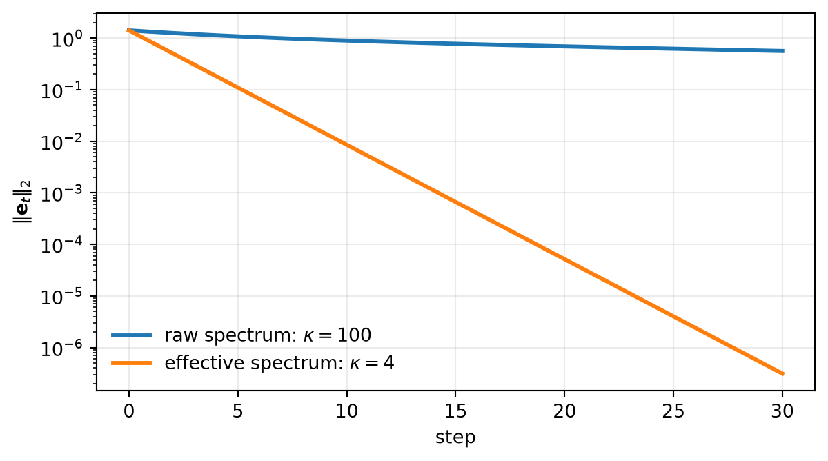
The next control does not use the oracle inverse. It scales the sharp coordinate by \(1/25\), changing effective eigenvalues \((1,100)\) into \((1,4)\).

1. Run thirty unscaled steps under the opening contract.
2. Declare a diagonal preconditioner and its effective spectrum.
3. Use the optimal scalar step for the compressed spectrum.
4. Compare error norms and assert the predicted separation.

# [1]
raw = quadratic_trace(
    hessian,
    initial_error,
    step_size=step_size,
    steps=30,
)

# [2]
preconditioner = np.diag([1.0, 1 / 25])
effective_eigenvalues = np.linalg.eigvalsh(preconditioner @ hessian)
effective_kappa = effective_eigenvalues[-1] / effective_eigenvalues[0]

# [3]
compressed_step = 2 / effective_eigenvalues.sum()
compressed = quadratic_trace(
    hessian,
    initial_error,
    step_size=compressed_step,
    steps=30,
    preconditioner=preconditioner,
)

# [4]
raw_norms = np.linalg.norm(raw.iterates, axis=1)
compressed_norms = np.linalg.norm(compressed.iterates, axis=1)
assert np.isclose(effective_kappa, 4.0)
assert compressed.final_error_norm < 1e-6
assert raw.final_error_norm > 0.5

fig, ax = plt.subplots(figsize=(7.0, 3.7))
ax.semilogy(raw_norms, linewidth=2.2, label=r"raw spectrum: $\kappa=100$")
ax.semilogy(
    compressed_norms,
    linewidth=2.2,
    label=r"effective spectrum: $\kappa=4$",
)
ax.set(xlabel="step", ylabel=r"$\|\mathbf{e}_t\|_2$")
ax.grid(alpha=0.25)
ax.legend(frameon=False)
plt.show()

print(
    f"effective eigenvalues={effective_eigenvalues.tolist()}, "
    f"kappa={effective_kappa:g}, step={compressed_step:g}"
)
print(
    f"step 30: raw norm={raw.final_error_norm:.6f}, "
    f"preconditioned norm={compressed.final_error_norm:.9f}"
)

Figure 4.2: A declared diagonal preconditioner compresses the effective spectrum from condition number 100 to 4. After 30 iterations the raw error norm is about 0.564, while the preconditioned error is about 3.13e-7. This is an exact quadratic model comparison; it does not establish the quality or cost of estimating a preconditioner in a changing problem.

effective eigenvalues=[1.0, 4.0], kappa=4, step=0.4
step 30: raw norm=0.564028, preconditioned norm=0.000000313

NoteField note: count the cost of the repair

An iteration reduction is not yet a wall-clock speedup. Applying or estimating \(\matr{P}\) moves bytes and performs work. The book will not convert a condition number into accelerator time without a hardware contract.

4.5 A stochastic update has no point endpoint

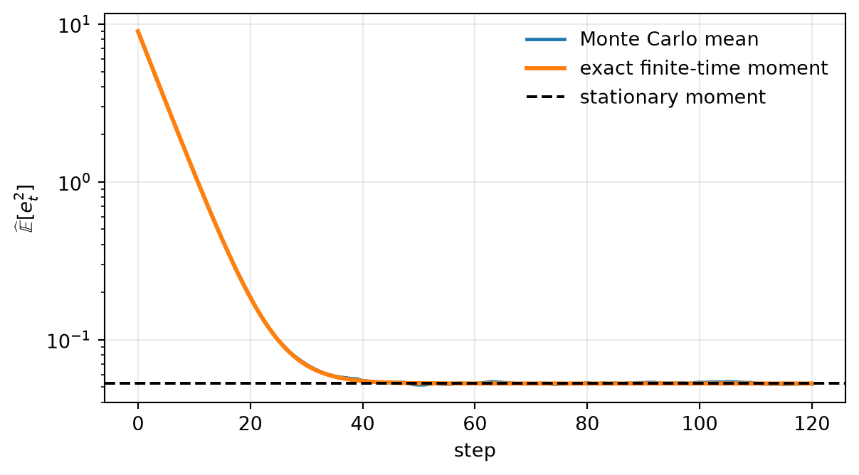
Now isolate one scalar mode of curvature \(\lambda>0\). Suppose the observed gradient contains additive noise:

\[ e_{t+1} = (1-\alpha\lambda)e_t-\alpha\xi_t, \qquad \E[\xi_t]=0, \qquad \E[\xi_t^2]=\tau^2. \tag{4.8}\]

The noise is independent across time and independent of the current state. These assumptions are the model, not decorative caveats.

Theorem 4.3 (Exact second moment under additive noise) If \(|1-\alpha\lambda|<1\), then

\[ \E[e_t^2] = (1-\alpha\lambda)^{2t}e_0^2 + \frac{\alpha\tau^2}{\lambda(2-\alpha\lambda)} \left[ 1-(1-\alpha\lambda)^{2t} \right]. \tag{4.9}\]

Consequently,

\[ \lim_{t\to\infty}\E[e_t^2] = \frac{\alpha\tau^2}{\lambda(2-\alpha\lambda)}. \tag{4.10}\]

Proof

Let \(r=1-\alpha\lambda\). Squaring Equation 4.8 and taking expectations removes the cross term by independence and zero mean:

\[ \E[e_{t+1}^2] = r^2\E[e_t^2]+\alpha^2\tau^2. \]

Unrolling the scalar recurrence gives

\[ \E[e_t^2] = r^{2t}e_0^2 + \alpha^2\tau^2\sum_{j=0}^{t-1}r^{2j}. \]

The geometric sum is \((1-r^{2t})/(1-r^2)\), and \(1-r^2=\alpha\lambda(2-\alpha\lambda)\). Substitution proves the result. \(\square\)

1. Simulate independent noisy scalar trajectories.
2. Estimate mean squared error over the trial axis.
3. Compute the exact finite-time and stationary predictions.
4. Assert agreement using the endpoint standard error.
5. Plot the transient and the floor.

# [1]
noisy = scalar_noisy_quadratic_trials(
    curvature=1.0,
    step_size=0.1,
    noise_standard_deviation=1.0,
    initial_error=3.0,
    steps=120,
    trials=20_000,
    seed=6213,
)

# [2]
estimated_mse = noisy.mean_squared_error
endpoint_se = noisy.endpoint_standard_error

# [3]
time = np.arange(121)
noise_factor = 1 - noisy.step_size * noisy.curvature
stationary = noisy.stationary_second_moment
predicted_mse = (
    noise_factor ** (2 * time) * noisy.initial_error**2
    + stationary * (1 - noise_factor ** (2 * time))
)

# [4]
assert abs(estimated_mse[-1] - predicted_mse[-1]) < 4 * endpoint_se

# [5]
fig, ax = plt.subplots(figsize=(7.0, 3.7))
ax.semilogy(time, estimated_mse, linewidth=1.8, label="Monte Carlo mean")
ax.semilogy(time, predicted_mse, linewidth=2.2, label="exact finite-time moment")
ax.axhline(stationary, color="black", linestyle="--", label="stationary moment")
ax.set(xlabel="step", ylabel=r"$\widehat{\mathbb{E}}[e_t^2]$")
ax.grid(alpha=0.25)
ax.legend(frameon=False)
plt.show()

print(
    f"endpoint MSE={estimated_mse[-1]:.8f}, "
    f"SE={endpoint_se:.8f}"
)
print(
    f"finite-time prediction={predicted_mse[-1]:.8f}, "
    f"stationary={stationary:.8f}"
)

Figure 4.3: Across 20,000 independent trials, the estimated squared error approaches the exact finite-time prediction and the stationary value 0.05263. The figure supports the additive, independent, finite-variance model in Equation 4.8; it does not establish a universal stochastic-gradient floor.

endpoint MSE=0.05229016, SE=0.00052526
finite-time prediction=0.05263158, stationary=0.05263158

This floor is algorithmic. C03’s stalled update was representational. A coordinate can also appear stationary because its deterministic multiplier is near one. These diagnoses require different controls:

Symptom	Instrument	Supported diagnosis
coordinate alternates sign	signed eigencoordinate	negative stable mode factor
coordinate decays very slowly	\(|1-\alpha\lambda_k|\)	conditioning tax
mean squared error plateaus across independent trials	estimator plus exact recurrence	stochastic floor under the declared model
requested change is below a local midpoint	local ULP audit	finite-grid stagnation
measured time remains large after iteration count falls	bytes/work profile	implementation cost

The scalar model keeps \(\tau^2\) and the curvature fixed, so it cannot diagnose when a stochastic run changes regime. C13 is obligated to replace \(\xi_t\) by a declared conditional gradient estimator, compare gradient signal with estimator variation, and test what happens when the second moment is not finite.

The fixed boundary in Equation 4.4 is now a registered control. C16 is obligated to compare it with local top curvature, curvature in the current gradient direction, and a setting in which the curvature itself moves during training.

TipCheck yourself

For eigenvalues \((2,20)\) and step \(\alpha=0.075\), what are both mode factors? How do you classify their sign behavior, which is the slow mode, and does reducing the step to \(0.025\) remove oscillation, improve the slowest contraction, both, or neither?

4.6 Okay, so —

• Inherited: C03 taught us to separate a missing update from a representational failure; basic gradient mechanics are assumed.
• Changed: A gradient trajectory is now an operator recurrence with a separate clock in every eigendirection.
• Instrumented: The harness records spectra, mode factors, exact quadratic traces, preconditioned traces, and stochastic second moments.
• Established: The stability interval, optimal constant-step contraction, and additive-noise floor follow exactly under their stated models.
• Unresolved: What probabilistic control survives when there are many possible directions and the stochastic perturbation is not fixed, additive, or light-tailed?

4.7 Sources and further reading

Nesterov develops gradient methods for smooth, strongly convex objectives and the role of conditioning (Nesterov 2004). Robbins and Monro supply the foundational stochastic-approximation setting (Robbins and Monro 1951). This chapter uses those sources as context, but derives its three exact recurrences on the page. Schmidt’s ICML 2026 tutorial motivates the global, local, directional, and finite-horizon questions used to delimit “best” (Schmidt 2026); it is an intellectual map, not the technical authority for the equations.

Reading order. Start with Nesterov (2004) for the fixed smooth, strongly-convex control, then read Robbins and Monro (1951) for the stochastic branch and Schmidt (2026) for the research-question map.

4.8 Exercises

1. (Pencil.) Mode phase diagram. For a scalar curvature \(\lambda\), draw the five regimes of \(1-\alpha\lambda\) as a function of \(\alpha\). Mark monotone decay, one-step annihilation, oscillatory decay, boundary behavior, and divergence.

2. (Pencil.) Bits and conditioning. Starting from Equation 4.5, derive an exact ceiling formula for the number of iterations required to reduce every eigencoordinate by a factor \(2^{-b}\). Then give its large-\(\kappa\) approximation and state where the approximation enters.

3. (Code.) A misleading loss curve. Construct two quadratic trajectories whose scalar objective curves are nearly indistinguishable for 50 steps but whose signed eigencoordinates have different mode classifications. Report the spectra and the control that separates them.

4. (Code.) Imperfect preconditioning. Sweep the second diagonal entry of \(\matr{P}=\operatorname{diag}(1,p)\) for the opening Hessian. For each value, choose the optimal constant step for the effective spectrum and report iteration count, matrix-application cost model, and final error.

5. (Audit.) The precision diagnosis. A report says, “The flat coordinate stopped changing, so the optimizer reached its noise floor.” List the eigencoordinate, repeated-trial, and local-ULP controls required before that conclusion is admissible. Predict what each rival explanation would do under those controls.

6. (Audit.) Paper audit: stochastic approximation. Complete the Claim, Resolution of the theory, Dynamic regime, Evidence culture and interface, and Assumption stress test fields for Robbins and Monro’s primary paper. Identify which step-size, noise, and convergence claims differ from the constant-step finite recurrence in this chapter. Label each extracted result as theorem, asymptotic statement, or heuristic interpretation.

7. (Audit.) Act checkpoint — open an Incident Card. Complete the Act 0 assignment for a numerical or performance failure. Fill Symptom, Prediction, Contract, Precision control, and Corrective control before reading the result. Route: Act checkpoint. Estimated time: 60 minutes. Deliverable: a partial card and one paired rerun. Hint: a speedup without a traffic boundary and a reduction over the wrong axis are different contract failures.

Nesterov, Yurii. 2004. Introductory Lectures on Convex Optimization: A Basic Course. Vol. 87. Applied Optimization. Kluwer Academic Publishers. https://doi.org/10.1007/978-1-4419-8853-9.

Robbins, Herbert, and Sutton Monro. 1951. “A Stochastic Approximation Method.” The Annals of Mathematical Statistics 22 (3): 400–407. https://doi.org/10.1214/aoms/1177729586.

Schmidt, Mark. 2026. Is Numerical Optimization Theory Irrelevant to Machine Learning Practice in 2026? Tutorial at the 43rd International Conference on Machine Learning. https://www.cs.ubc.ca/~schmidtm/Documents/2026_ICML_Tutorial.pdf.