A copy performs no arithmetic. A fused affine transform performs \(2N\) operations. Their compulsory traffic — and therefore their bandwidth time bound — is the same.
Both computations act on \(N\) stored FP32 values. The copy moves at least \(8N\) bytes: one read and one write. The fused transform \(y_i=ax_i+b\) has the same dominant traffic when \(a\) and \(b\) remain in a fast store. One operation count is zero; that count does not identify elapsed time.
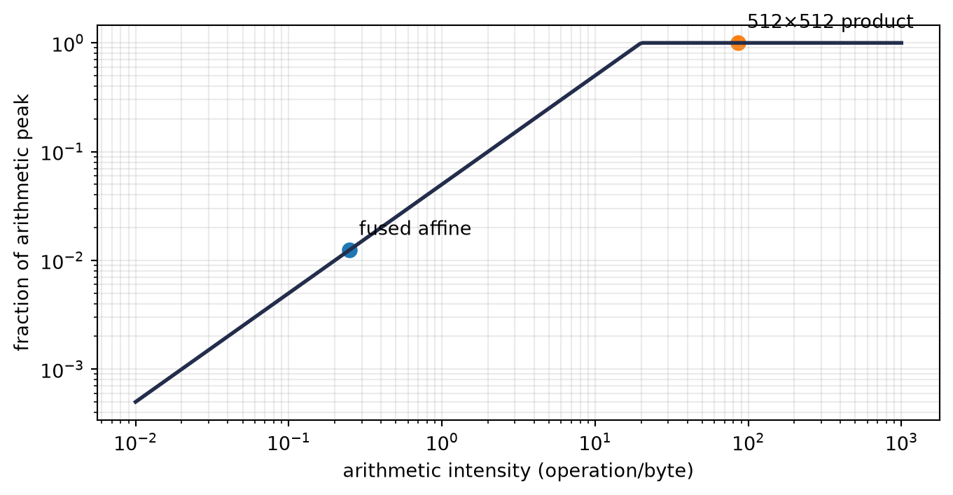
Now compare a square matrix product of order \(n=512\). The conventional count is \(2n^3\) operations. Its compulsory traffic under an idealized one-read, one-write model is \(12n^2\) bytes, so its arithmetic intensity is \(n/6=85.33\) operations per byte. The affine transform has intensity \(2/8=0.25\). On a hypothetical machine whose peak arithmetic-to-bandwidth ratio is 20, one falls below the balance point and the other lies above it. The larger operation count can be the computation with more opportunity to reuse data.
ImportantPrediction
On one fixed machine, a proposed method halves the multiplications and doubles compulsory traffic. Choose a prediction before continuing: faster, slower, or undetermined. Which traffic boundary and machine balance would let you defend that choice?
1.1 Two resource clocks
Let \(F\) be the required operations, \(Q\) the bytes transferred through a declared boundary, \(P_{\max}\) peak arithmetic rate, and \(B\) peak bandwidth. The two unavoidable time lower bounds are
With arithmetic intensity \(I=F/Q\), achieved performance \(P=F/T\) obeys the following deliberately small theorem.
Theorem 1.1 (Two-resource performance ceiling) Under the declared operation count, traffic boundary, peak arithmetic rate, and peak bandwidth,
\[
P\leq \min(P_{\max},BI).
\tag{1.2}\]
Proof
Invert each inequality in Equation 1.1 and multiply by \(F\). The arithmetic bound gives \(P\leq P_{\max}\); the traffic bound gives \(P\leq BF/Q=BI\). Both must hold.
The bend occurs at the machine balance\(I_*=P_{\max}/B\). This diagram is the roofline model (Williams et al. 2009). It is an upper envelope, not a prediction that a kernel reaches either roof.
Read the committed C01 model calculation.
Declare one hypothetical machine balance.
Plot the bandwidth and arithmetic ceilings.
Place the vector transform and matrix product on the same axes.
Check the registered arithmetic intensities before interpretation.
Figure 1.1: One operation count is not one cost. Under the declared two-resource model, the vector transform lies below the balance point while the reused matrix product lies above it.
1.2 A zero-count kernel still consumes a clock
The model now needs a measured control. The committed observation times a 64 MiB FP32 payload copy and an order-512 FP32 matrix product on one Apple M4 Max CPU. It also sweeps nearby sizes to establish two local empirical ceilings in the same process. Those ceilings are not vendor peaks. They are reference rates that make the achieved fractions inspectable without claiming that a laptop CPU represents an accelerator.
Read the pinned local measurement and its protocol.
Extract the selected copy and matrix-product rates.
Normalize each rate by its own local empirical ceiling.
Plot resource-specific fractions rather than a false common unit.
Check that the displayed values match the committed observation.
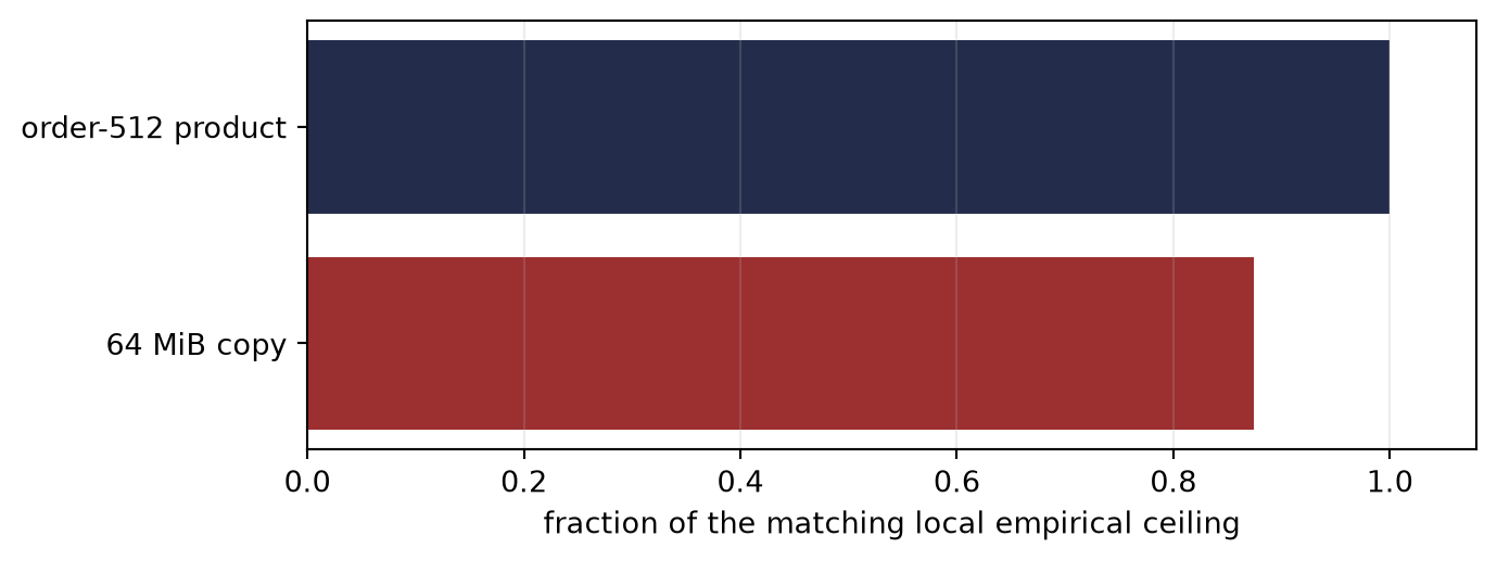
Figure 1.2: A zero-FLOP copy has a positive measured cost. Each bar is normalized by a separately measured local ceiling for its own resource, so the figure supports a resource diagnosis rather than a cross-kernel speed ranking.
The copy moved a 64 MiB payload across the declared read-plus-write boundary, so the traffic count was 128 MiB. Its median time was about \(0.947\) ms and its achieved bandwidth was \(141.7\) GB/s, or \(87.5\%\) of the best copy rate in the declared size sweep. The matrix product reached \(2581.6\) GFLOP/s in the same software process. These observations do not say that one kernel is generally faster: they show that zero counted arithmetic does not mean zero elapsed time, and that each kernel must be compared with the roof for the resource it actually demands.
1.3 The denominator is an algorithmic choice
Traffic has no meaning until its boundary is named. Bytes between registers and a first-level cache, between cache and main memory, and between host and accelerator are different denominators. Tiling changes \(Q\) by retaining a working set near arithmetic units. Fusion changes \(Q\) by keeping an intermediate value from making a round trip. Recompute can deliberately increase \(F\) to reduce \(Q\). C11 will return to exactly that trade when it checkpoints derivative state.
This also foreshadows the numerical-stability thread that C02 seeds. A fused operation can change both traffic and rounding: eliminating an intermediate store may eliminate one rounding step. A performance transformation is therefore part of the numerical contract, not merely a scheduling detail.
WarningNamed wrong answer: fewer operations means faster
Fewer operations is evidence only after the limiting resource is identified. It may improve a compute-limited kernel, do nothing to a bandwidth-limited kernel, or make the kernel slower by destroying reuse or fusion.
1.4 Hardware-claim boundary
The roofline is useful because it makes omissions visible. Peak values may be unreachable; compulsory traffic can underestimate actual traffic; latency, launch overhead, synchronization, occupancy, instruction mix, and access regularity remain outside Equation 1.2. CPU simulation of FP16 behavior is not evidence of accelerator timing. Any measured claim later in this book must name the device, software stack, warmup, repetitions, statistic, and traffic boundary—or be labeled a model calculation or pinned artifact.
TipField note: read a speedup claim in three passes
First locate the mathematical work and the denominator behind its reported rate. Then locate the resource boundary: bytes, arithmetic, latency, communication, or some mixture. Only then compare measured elapsed time, including baseline, device, precision, warmup, repetitions, statistic, and failure accounting. A speedup is an observation about that full comparison, not a synonym for a smaller operation count.
1.5 Check yourself
A kernel performs \(10^{10}\) operations and moves \(10^9\) bytes. On a device with \(P_{\max}=10^{13}\) operation/s and \(B=5\times10^{11}\) byte/s, its intensity is what? What are the machine balance, active roofline branch, and model ceiling? If \(F\) is halved while \(Q\) is unchanged, which lower bound changes and which one does not?
Changed: elapsed-time reasoning now requires a declared traffic denominator and machine balance.
Instrumented: one exact roofline claim and one pinned laptop measurement separate modeled ceilings from achieved rates.
Established:\(P\leq\min(P_{\max},BI)\) follows from two resource lower bounds.
Unresolved: Which state must an online computation retain when real executions move data through multiple memory levels?
1.7 Sources and further reading
The roofline formulation and its machine-balance interpretation follow Williams et al. (2009). For systems-scale companions that carry rooflines into accelerator topology, collectives, and large-model execution, see Austin et al. (2025) and Tazi et al. (2025).
Reading order. Start with Williams et al. (2009) for the two-resource diagram, then return to this chapter’s denominator and measurement sections before using Austin et al. (2025) or Tazi et al. (2025) for multi-device scale.
1.8 Exercises
(Pencil.) Recompute the matrix-product intensity if one input matrix is reread four times. State the traffic boundary.
(Code.) For three hypothetical machine balances, redraw the figure and report which classifications change. Do not time the plotting code.
(Pencil.) A checkpointing rule adds \(30\%\) arithmetic and removes half the retained-state traffic. Derive the intensities before and after, then state the machine-balance range in which the trade can improve the roofline bound.
(Code.) Re-run the local protocol with three payload sizes and three matrix orders. Declare device, stack, warmup, repetitions, statistic, and traffic boundary. Compare medians and dispersion; do not call the best observed rate a vendor peak.
(Audit.) Paper audit: Find one reported speedup and complete the Claim, Mathematical object, Evidence culture and interface, Numerical and hardware contract, and Transfer verdict fields of the Paper Autopsy Protocol. Separate operation count, modeled traffic, measured elapsed time, hardware identity, and baseline. Which claim is actually supported?
Austin, Jacob, Sholto Douglas, Roy Frostig, et al. 2025. How to Scale Your Model: A Systems View of LLMs on TPUs. Online book. https://jax-ml.github.io/scaling-book/.
Williams, Samuel, Andrew Waterman, and David Patterson. 2009. Roofline: An Insightful Visual Performance Model for Multicore Architectures. UCB/EECS-2008-134. University of California, Berkeley. https://digicoll.lib.berkeley.edu/record/136692.