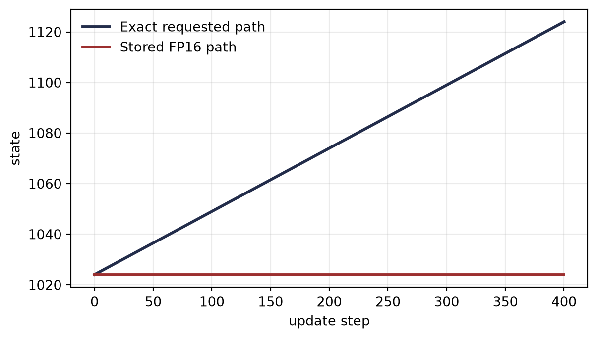
A parameter is stored as FP16 at the value \(1024\). An algorithm asks for the same update, \(+0.25\), four hundred times. Exact arithmetic ends at \(1124\). The stored parameter never moves.
Nothing overflowed. The update was not zero. The code executed all four hundred additions. Yet every requested change disappeared.
ImportantPrediction
Which boundary swallowed the update?
The value left the format’s range.
The input \(0.25\) could not be represented.
The addition produced a result that rounded back to \(1024\).
Positive and negative quantities catastrophically cancelled.
Choose one, then name the control that would separate it from the others.
3.1 The update that never lands
The opening witness is a format simulation on a CPU. It makes a statement about FP16 rounding, not about CPU or accelerator speed. The chapter verifies and imports its own vendored harness wheel, so later changes to the package cannot silently alter this result.
Load the chapter-pinned precision instruments.
Request four hundred \(+0.25\) updates from the same initial value.
Record the local spacing and the full precision contract.
Assert the stalled stored path against the exact path.
Figure 3.1: A requested update of 0.25 advances the exact trajectory but never changes an FP16 value stored at 1024. The figure supports a local-resolution diagnosis under the declared round-after-each-step contract; it is not a hardware timing result.
harness=ch-03 wheel=833cfe618f0c
local spacing=1; half spacing=0.5
exact endpoint=1124; stored endpoint=1024
The value \(0.25\) is exactly representable in binary. The exact sum \(1024.25\) is also far inside the finite range of FP16. The failure occurs when that sum must be stored back on the local FP16 grid. Its neighbors are \(1024\) and \(1025\); round-to-nearest returns \(1024\). The next step starts from the same state and repeats the same loss.
This is stagnation by local resolution. Describing the computation only as “FP16” does not reveal it. We needed the state value, update size, storage point, and rounding rule.
3.2 A floating format is a changing grid
A normalized radix-two value with \(p\) significand bits has the form
\[
x
=
\pm\left(1.b_1b_2\cdots b_{p-1}\right)_2 2^e.
\tag{3.1}\]
The leading one is fixed for normal values. Incrementing the last stored bit changes the significand by \(2^{-(p-1)}\), then the exponent scales that change by \(2^e\).
Theorem 3.1 (Binade spacing) In a normalized radix-two format with \(p\) significand bits, consecutive representable values in the binade \([2^e,2^{e+1})\) differ by
\[
\Delta_e=2^{e-(p-1)}.
\tag{3.2}\]
Under round-to-nearest, an update from a representable value cannot change the stored result unless the exact result reaches a midpoint between grid points, with the midpoint itself decided by the tie rule.
Proof
Within one binade, the exponent \(e\) is fixed. The stored significands are
Round-to-nearest assigns every exact value between two adjacent midpoints to the enclosed grid point. A smaller perturbation cannot cross that cell’s boundary. \(\square\)
For FP16, \(p=11\). At \(1024=2^{10}\), Equation 3.2 gives
\[
\operatorname{ulp}(1024)=2^{10-(11-1)}=1.
\]
The update \(0.25\) is only one quarter of the local spacing and one half of the distance to the rounding boundary.
Three nearby quantities that are not synonyms
\(\operatorname{ulp}(x)\) is a local grid spacing near \(x\).
Machine epsilon, \(\varepsilon_{\mathrm{mach}}\), is the gap from \(1\) to the next larger representable value.
For round-to-nearest in a normal binade, the unit roundoff is \(u=\varepsilon_{\mathrm{mach}}/2\).
The conventional one-operation model is
\[
\operatorname{fl}(z)=z(1+\delta),
\qquad |\delta|\le u.
\tag{3.3}\]
It applies when one exact result \(z\) is correctly rounded to a normal finite value. It is not a license to ignore overflow, gradual underflow, multiple operations, an already-rounded input, or an unspecified reduction.
WarningNamed wrong answer: ‘Machine epsilon is the smallest number the format can store’
Machine epsilon describes the gap after one. The smallest positive normal and the smallest positive subnormal describe range near zero. Local spacing grows with the exponent. One number cannot stand in for all three.
3.3 Range and resolution are separate budgets
The next instrument queries the format instead of relying on remembered decimal approximations.
Query the FP16 and FP32 format contracts at runtime.
Separate significand allocation from exponent allocation.
Report epsilon, unit roundoff, and both lower range boundaries.
FP16: significand=11 bits, exponent=5 bits
FP32: significand=24 bits, exponent=8 bits
FP16: eps=0.0009765625, u=0.00048828125
  normal floor=6.1035156e-05, smallest subnormal=5.9604645e-08, largest finite=65504
FP32: eps=1.1920929e-07, u=5.9604645e-08
  normal floor=1.1754944e-38, smallest subnormal=1.4012985e-45, largest finite=3.4028235e+38
Increasing exponent bits extends the range; increasing significand bits refines the grid within a binade. Those are different resources. A value can be finite but too coarsely resolved for the update applied to it. Conversely, a computation can have fine relative resolution throughout its normal range and still overflow because that range is too short.
Subnormal values extend the grid below the smallest normal with reduced relative precision. A system may also change their execution behavior. The portable claim is therefore not merely a smallest-positive number: the contract must say whether subnormals are supported or flushed.
NoteField note: a dtype name leaves four blanks
Record storage, compute, accumulation, and output dtypes separately. Then record the rounding rule and exceptional-value behavior. A reduction can read narrow operands, multiply in one format, accumulate in a wider format, and round to a narrow output. Calling the entire path “FP16” hides the operation most likely to fail.
This chapter simulates the declared rounding contract on a CPU. It never uses CPU FP16 timing as evidence about accelerator performance.
3.4 Two losses that no longer look alike
Chapter 2 separated two failures:
distinctions can disappear when real inputs are represented on a grid;
represented inputs can survive, while the evaluation path destroys the desired result.
Local spacing now makes the first boundary quantitative. If two real values round to the same stored value, no later algorithm can infer which one arrived. Wider accumulation begins too late.
Cancellation is different. Suppose \(x\) and \(y\) are close, but the represented operands satisfy
\[
\widehat{x}=x(1+\delta_x),
\qquad
\widehat{y}=y(1+\delta_y),
\qquad
|\delta_x|,|\delta_y|\le u.
\]
Theorem 3.2 (Cancellation amplification) If \(x\ne y\), then even before rounding the subtraction itself,
Divide by the nonzero exact difference \(|x-y|\). \(\square\)
When \(|x-y|\) is tiny compared with \(|x|+|y|\), the subtraction exposes errors that were small relative to the operands but large relative to the answer. Performing that final subtraction in a wider format does not restore bits already lost while the two operands were formed.
This closes the first promise from Chapter 2. Its raw moments occupied the scale of \(\mu^2\), and their rounded values differed by exactly one \(\operatorname{ulp}(\mu^2)=32\). The impossible variance was therefore \(-32\), while the centered algorithms avoided constructing those two large nearby operands. At a still larger offset, distinct deviations eventually map to the same FP32 input; that later representation loss is irrecoverable.
The bound in Equation 3.4 is a diagnostic sensitivity statement. It does not include the addition count, reduction tree, fused operations, or accumulator format of a complete kernel. Those belong in the precision contract.
3.5 Resolution must be allocated
A finite grid is not merely chosen; it is placed. Consider a signed \(b\)-bit symmetric integer grid with
One scale for \([0.1,0.2,0.3,100]\) must cover the outlier. The following model uses eight signed bits. It is a uniform integer quantizer, not a floating-point format.
Quantize all four coordinates with one declared symmetric scale.
Quantize the first three coordinates as one block and the outlier as another.
Compare integer codes and reconstructed values.
Assert that only the global scale erases every small coordinate.
The global step is 0.787402; every small coordinate lies below half that step and rounds to zero. The first block’s step is 0.002362, so those coordinates receive useful codes. Nothing about the bit count alone predicted the difference. Scale granularity was part of the algorithm.
Blocking is not free. It stores more scales, adds grouping rules, and can introduce discontinuities at block boundaries. The supported conclusion is not that smaller blocks are always better. It is that a claim about quantization error is incomplete until scale selection and block axes are specified.
3.6 Changing the rounding rule
The opening update is always pushed toward the old state by deterministic rounding. A different rounding rule can remove that one-sided local error.
Let \(a<x<b\) be adjacent grid points. Define stochastic adjacent rounding by
Because the mean error is zero, this second moment is also the variance. \(\square\)
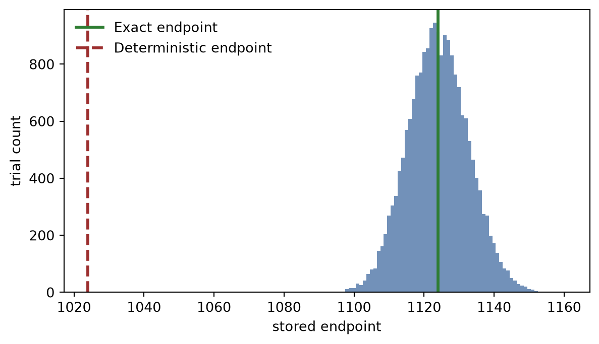
At the opening state, each requested value is an integer plus \(0.25\) and the grid spacing remains one. Each step therefore moves upward with probability \(0.25\). Under independent draws, the endpoint has the model
\[
1024+\operatorname{Binomial}(400,0.25),
\]
with mean \(1124\) and standard deviation \(\sqrt{400(0.25)(0.75)}\approx 8.66\).
Run seeded stochastic-rounding trials under the opening contract.
Estimate the endpoint mean, standard deviation, and standard error.
Compare the mean with the exact endpoint and the binomial model.
Plot the endpoint distribution with both reference locations.
Figure 3.2: Across 20,000 seeded trials, stochastic adjacent rounding centers the endpoint distribution near the exact endpoint 1124, whereas deterministic rounding ends at 1024. The figure supports an expectation claim for this declared model, not exact trajectories or general training convergence.
mean=1124.00655, sd=8.64855, SE(mean)=0.06115
normal 95% interval for mean=[1123.88669, 1124.12641]
The estimated mean is 1124.00655, with standard error 0.06115. The exact endpoint lies inside the displayed normal-approximation interval for the mean. Individual trajectories remain noisy; their standard deviation is about 8.65.
WarningNamed wrong answer: ‘Unbiased rounding makes the training run unbiased’
The theorem concerns one rounding event conditional on its input. A later state depends on earlier random outcomes, and nonlinear maps do not generally preserve unbiasedness. Stochastic rounding prevents this deterministic sub-grid stagnation in expectation. It does not prevent overflow, choose a good scale, stabilize an update rule, or guarantee convergence.
3.7 Diagnose before prescribing
The same symptom—no visible progress—admits different repairs.
Diagnostic
Instrument
Matched repair
Repair cannot do
Value exceeds range
Peak and exceptional-value trace
Rescale, widen exponent range, or change the evaluation
Recover an overflowed intermediate after the fact
Update lies below local midpoint
\(\operatorname{ulp}(w)\) versus \(|\Delta w|\)
Retain a wider state, rescale, accumulate increments, or use a scoped rounding change
Make the mathematical update direction correct
Inputs already coincide on the grid
Same-input wider reference
Change upstream storage or scaling
Infer distinctions absent from the input
Nearby large operands expose prior errors
Cancellation ratio and wider controls
Reformulate or form operands more accurately
Repair arbitrary ill-conditioning
One outlier sets a global quantization step
Per-block maxima and zero-code rate
Allocate scales by a declared block or channel
Eliminate scale metadata and boundary costs
Long reduction loses increments
Accumulator dtype and reduction-order audit
Widen or compensate the accumulation
Establish accelerator speed from CPU timing
This table is the precision language promised by Chapter 2. The dtype is one field inside the diagnosis, not the diagnosis itself.
The same discipline will return in later acts. A variance-preserving initialization must keep values in range as well as control exact moments. Batch-coordinate normalization inherits the centered-state estimator and its accumulator contract. An edge-of-stability trace needs a precision control before a spike is assigned to curvature. A quantized update must declare where its scale came from.
TipCheck yourself
A stored parameter is \(2048\) in FP16 and a computation requests \(+0.75\). Without running code, compute the local spacing, identify the two adjacent stored candidates, and predict the round-to-nearest result. Which part of the answer would change under stochastic adjacent rounding?
3.8 Okay, so —
Inherited: Chapter 2 showed that algebraically equal formulas can have different execution behavior and that wider downstream arithmetic cannot reconstruct absent inputs.
Changed: “FP16” is no longer an explanation. The operative object is a contract over storage, compute, accumulation, output, rounding, range, and scale.
Instrumented: The harness now measures local spacing, queries format envelopes, simulates round-after-each-step trajectories, audits block quantizers, and estimates stochastic endpoints with uncertainty.
Established: Binade spacing predicts the stalled update; cancellation amplifies operand errors relative to a small difference; stochastic adjacent rounding is locally unbiased with an exact error variance.
Unresolved: Is an observed training failure numerical, dynamic, or geometric, and which control separates those explanations?
3.9 Sources and further reading
IEEE 754 specifies floating-point formats and operations (IEEE Standard for Floating-Point Arithmetic 2019). Higham develops the standard rounding model, cancellation, stability, and error analysis in detail (Higham 2002). Connolly, Higham, and Mary analyze stochastic rounding and its probabilistic backward-error behavior (Connolly et al. 2021). The FP8 proposal by Micikevicius and collaborators is useful modern format context, but it does not make a format name a complete execution contract (Micikevicius et al. 2022).
The Probabilistic Numerics tutorial contrasts uncertainty from limited computation with uncertainty from limited data (Hennig et al. 2026). Exercise 7 uses that analogy as an audit boundary: neither a deterministic rounding bound nor local unbiasedness is automatically a calibrated posterior over an unfinished computation.
For introductory format anatomy, mixed-precision roles, and the hardware motivation, see the sibling volume’s precision and hardware appendix. This chapter owns the local-grid diagnosis, the cancellation boundary, resolution allocation, and the rounding-rule audit.
Reading order. Start with Higham (2002) for the error-analysis language, consult (IEEE Standard for Floating-Point Arithmetic 2019) for the exact format contract, and then use Connolly et al. (2021) to audit what stochastic rounding changes.
3.10 Exercises
(Pencil.) Binade boundaries. For FP16, compute the spacing immediately below \(2^{10}\), at \(2^{10}\), and at \(2^{11}\). Explain why \(\operatorname{ulp}(x)\) jumps at a power of two even though relative precision remains of the same order.
(Pencil.) Cancellation control. Let \(x=1+\eta\) and \(y=1\), with \(\eta>0\). Use Equation 3.4 to identify the amplification factor. Then explain why the bound diagnoses sensitivity without predicting the exact sign of the error.
(Code.) Stagnation map. Sweep represented FP16 states across several binades and requested positive updates. Predict stagnation from the local midpoint before running the harness. Report a confusion matrix between the prediction and observed state changes.
(Code.) Scale allocation. Add one adjustable outlier to a vector of small coordinates. Compare global, fixed-block, and per-coordinate symmetric scales using reconstruction error and zero-code rate. Count scale metadata explicitly; do not rank methods on error alone.
(Audit.) The incomplete precision claim. A report says, “The model was trained in FP16 and remained stable.” Write the missing storage, compute, accumulation, output, rounding, exceptional-value, and scaling questions. For each question, name one rival explanation it could eliminate.
(Audit.) Paper audit: FP8 formats. Complete the Claim, Mathematical object, Evidence culture and interface, Numerical and hardware contract, and Transfer verdict fields for the primary FP8 format proposal cited above. Extract one claim about a format, one about an execution path, and one empirical result. For each, record its assumptions and identify whether the paper’s evidence is a proof, model calculation, simulation, or hardware measurement. Do not convert a paper-reported endpoint into a reproduced book claim.
(Audit.) Computational uncertainty. Compare three objects: a deterministic roundoff bound, stochastic adjacent rounding under the model in this chapter, and a probabilistic numerical posterior (Hennig et al. 2026). For each, record the source of randomness, what is conditioned on, what event the uncertainty statement covers, and what calibration evidence would be needed. Explain why local unbiasedness of a rounding error does not by itself quantify uncertainty in the exact computation.
Connolly, Michael P., Nicholas J. Higham, and Theo Mary. 2021. “Stochastic Rounding and Its Probabilistic Backward Error Analysis.”SIAM Journal on Scientific Computing 43 (1): A566–85. https://doi.org/10.1137/20M1334796.
Hennig, Philipp, Marvin Pförtner, and Tim Weiland. 2026. Probabilistic Numerics: Computation Is Machine Learning. Tutorial at the 43rd International Conference on Machine Learning. https://icml.cc/Downloads/2026.
Higham, Nicholas J. 2002. Accuracy and Stability of Numerical Algorithms. 2nd ed. Society for Industrial; Applied Mathematics. https://doi.org/10.1137/1.9780898718027.
Micikevicius, Paulius, Dusan Stosic, Neil Burgess, et al. 2022. “FP8 Formats for Deep Learning.”arXiv Preprint arXiv:2209.05433, ahead of print. https://doi.org/10.48550/arXiv.2209.05433.