12  Curvature Is Not One Matrix: Hessian, Generalized Gauss–Newton, Fisher, and Matrix-Free Products

RS · Random-matrix spectra · LG · Landscape and update geometry Geometric primary · Dynamic supporting · Algorithmic supporting

Take one Bernoulli observation with label \(y=1\). Let its logit be the composed map

\[ z(w)=w^2,\qquad \ell(w)=\log(1+e^{z(w)})-yz(w). \tag{12.1}\]

At \(w=1/2\), the predicted probability is \(p=\sigma(1/4)=0.5621765009\). Four quantities that are routinely called “curvature” give

\[ \begin{aligned} H &= -0.6295129155, &\qquad G &= 0.2461340827,\\ F &= 0.2461340827, &\qquad \widetilde F &= 0.1916894164. \end{aligned} \tag{12.2}\]

The first object says the realized loss bends downward. The other three are nonnegative. Two agree exactly; the third does not. No floating-point format, batch, parameter, or label changed. Only the mathematical question changed.

ImportantPrediction

Which term makes \(H\) negative? Why do \(G\) and \(F\) agree here? What distribution would have to change before \(\widetilde F\) became an empirical estimate of \(F\)?

12.1 Hold the problem fixed; change the object

The one-observation arithmetic is short enough to expose. For Bernoulli negative log likelihood,

\[ \frac{\partial\ell}{\partial z}=p-y,\qquad \frac{\partial^2\ell}{\partial z^2}=p(1-p). \tag{12.3}\]

Because \(z'(w)=2w\) and \(z''(w)=2\),

\[ \frac{d^2\ell}{dw^2} =\underbrace{p(1-p)[z'(w)]^2}_{G} +\underbrace{(p-y)z''(w)}_{\text{model-curvature term}}. \tag{12.4}\]

The first term is \(0.2461340827\). The second is \(-0.8756469982\). Their sum is the negative Hessian in Equation 12.2. The Fisher and empirical-Fisher values require different averaging contracts; they arrive in Section 12.3.

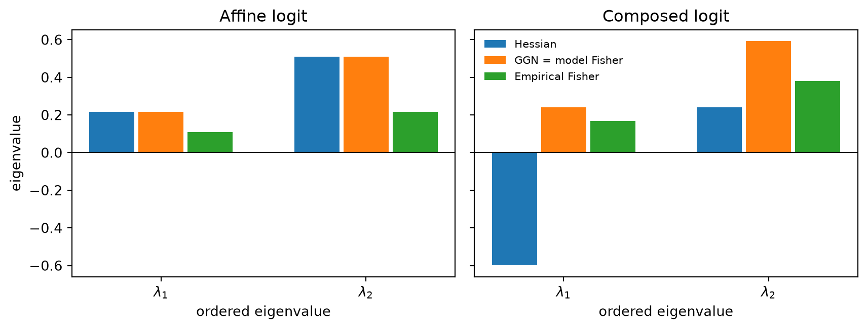
The next witness adds an intercept and four observations. It compares an affine logit \(z=ax+b\) with a composed logit \(z=a^2x+b\) while holding the parameter, labels, and Bernoulli loss fixed.

1. Load the chapter-pinned curvature instruments.
2. Fix four inputs, four labels, and one parameter vector.
3. Compute the realized Hessian, GGN, model Fisher, and empirical Fisher.
4. Repeat for affine and composed logits.
5. Compare eigenvalues rather than collapsing each matrix to one norm.
6. Check the committed claim artifact before interpreting the plot.

import matplotlib.pyplot as plt
import numpy as np

# [1]

from trainable_harness import bernoulli_curvature_matrices

# [2]
inputs = np.array([-2.0, -1.0, 1.0, 2.0])
labels = np.array([0.0, 0.0, 1.0, 1.0])
parameters = np.array([0.5, 0.0])

# [3]
def evaluate(nonlinear):
    return bernoulli_curvature_matrices(
        parameters,
        inputs,
        labels,
        nonlinear_first_parameter=nonlinear,
    )

affine = evaluate(False)

# [4]
composed = evaluate(True)

# [5]
objects = ("Hessian", "GGN = model Fisher", "Empirical Fisher")
fig, axes = plt.subplots(1, 2, figsize=(9.0, 3.5), sharey=True)
for axis, title, result in zip(
    axes,
    ("Affine logit", "Composed logit"),
    (affine, composed),
    strict=True,
):
    spectra = (
        np.linalg.eigvalsh(result.hessian),
        np.linalg.eigvalsh(result.generalized_gauss_newton),
        np.linalg.eigvalsh(result.empirical_fisher),
    )
    positions = np.arange(2)
    for offset, (name, spectrum) in enumerate(zip(objects, spectra, strict=True)):
        axis.bar(positions + 0.24 * (offset - 1), spectrum, 0.22, label=name)
    axis.axhline(0.0, color="black", linewidth=0.8)
    axis.set_xticks(positions, (r"$\lambda_1$", r"$\lambda_2$"))
    axis.set_title(title)
    axis.set_xlabel("ordered eigenvalue")
axes[0].set_ylabel("eigenvalue")
axes[1].legend(frameon=False, fontsize=8)
fig.tight_layout()

# [6]
claim = verify_claim("c12-curvature-choice-001", expected_harness=pin)
assert np.allclose(
    claim["result"]["composed_logit"]["hessian_eigenvalues"],
    np.linalg.eigvalsh(composed.hessian),
    atol=1e-12,
    rtol=0.0,
)
print("claim c12-curvature-choice-001: verified")

claim c12-curvature-choice-001: verified

Figure 12.1: The same Bernoulli loss produces different curvature spectra. With an affine logit, the realized Hessian, GGN, and model Fisher coincide. Curving the parameter-to-logit map adds an indefinite model-curvature term; the empirical Fisher remains a distinct observed-label outer product in both controls.

The affine control removes every Hessian of the parameter-to-logit map. The realized Hessian then equals GGN. The composed control restores one omitted term and one Hessian eigenvalue crosses zero. This is not a contest in which one matrix is universally correct. Each answers a different question.

12.2 The term a positive-semidefinite surrogate drops

Let \(f_{\vect{\theta}}\in\mathbb{R}^q\) be the model output, let \(\ell(y,\vect{z})\) be a local loss, and define \(\matr{J}=\partial f_{\vect{\theta}}/\partial\vect{\theta}\). Dimensions are \(\matr{J}\in\mathbb{R}^{q\times p}\) and \(\matr{H}_{\vect{z}}\ell\in\mathbb{R}^{q\times q}\).

Theorem 12.1 (Composite Hessian decomposition) If \(f_{\vect{\theta}}\) and \(\ell\) are twice differentiable, then

\[ \nabla_{\vect{\theta}}^2\ell =\underbrace{\matr{J}^{\mathsf T}\matr{H}_{\vect{z}}\ell\,\matr{J}}_{\matr{G}\text{: generalized Gauss--Newton}} +\underbrace{\sum_{j=1}^q \frac{\partial\ell}{\partial z_j} \nabla_{\vect{\theta}}^2 f_{\vect{\theta},j}}_{\matr{R}\text{: model curvature}}. \tag{12.5}\]

If \(\ell\) is convex in \(\vect{z}\), then \(\matr{G}\) is positive semidefinite. The residual term \(\matr{R}\) can have either sign.

Proof

The gradient is \(\nabla_{\vect{\theta}}\ell=\matr{J}^{\mathsf T} \nabla_{\vect{z}}\ell\). Differentiate its \(r\)-th coordinate with respect to \(\theta_s\). Differentiating \(\nabla_{\vect{z}}\ell\) produces \([\matr{J}^{\mathsf T}\matr{H}_{\vect{z}}\ell\matr{J}]_{rs}\); differentiating the entries of \(\matr{J}\) produces \(\sum_j(\partial\ell/\partial z_j) \partial^2 f_j/(\partial\theta_r\partial\theta_s)\). That is Equation 12.5. If \(\matr{H}_{\vect{z}}\ell\succeq0\), then \(\vect{v}^{\mathsf T}\matr{G}\vect{v}= (\matr{J}\vect{v})^{\mathsf T}\matr{H}_{\vect{z}}\ell (\matr{J}\vect{v})\geq0\).

The theorem explains both panels. In the affine model, \(\nabla^2_{\vect{\theta}} f_j=\matr{0}\) and \(\matr{R}=\matr{0}\). In the composed model, the observed residual multiplies the curvature of \(a^2x+b\).

WarningNamed wrong answer: GGN is the Hessian made safe

GGN is not the Hessian with negative eigenvalues clipped. It is the Hessian of a locally linearized model composed with the declared output loss. It can omit positive as well as negative model curvature, and it changes if the boundary between model and output loss changes.

12.3 Three expectations hiding behind two words

For a conditional statistical model \(p_{\vect{\theta}}(y\mid x)\), define the score \(\vect{s}_{\vect{\theta}}(y,x)=\nabla_{\vect{\theta}}\log p_{\vect{\theta}}(y\mid x)\). Fixing the observed inputs, the model Fisher is

\[ \matr{F}(\vect{\theta}) =\frac{1}{m}\sum_{i=1}^m \E_{Y\sim p_{\vect{\theta}}(\cdot\mid x_i)} \left[\vect{s}_{\vect{\theta}}(Y,x_i) \vect{s}_{\vect{\theta}}(Y,x_i)^{\mathsf T}\right]. \tag{12.6}\]

The expectation resamples the label from the current model. The empirical Fisher used in the opening instead keeps the observed label:

\[ \widetilde{\matr{F}}(\vect{\theta}) =\frac{1}{m}\sum_{i=1}^m \vect{s}_{\vect{\theta}}(y_i,x_i) \vect{s}_{\vect{\theta}}(y_i,x_i)^{\mathsf T}. \tag{12.7}\]

Both are positive semidefinite sums of outer products. That shared algebra does not make their averaging distributions the same.

Theorem 12.2 (Score identity and qualified GGN equality) Suppose the support of \(p_{\vect{\theta}}(y\mid x)\) does not depend on \(\vect{\theta}\) and differentiation may pass through its integral or sum. Then

\[ \E[\vect{s}_{\vect{\theta}}]=\vect{0},\qquad \E[\vect{s}_{\vect{\theta}}\vect{s}_{\vect{\theta}}^{\mathsf T}] =-\E[\nabla_{\vect{\theta}}^2\log p_{\vect{\theta}}]. \tag{12.8}\]

When the output variable in the GGN is a compatible natural parameter for the negative log likelihood, the model Fisher equals that GGN.

Proof of the score identity

Differentiate normalization: \(\int p_{\vect{\theta}}(y\mid x)\,dy=1\). The first derivative gives \(\E[\vect{s}_{\vect{\theta}}]=\vect{0}\). Differentiating the score mean once more gives

\[ \vect{0} =\E[\nabla_{\vect{\theta}}^2\log p_{\vect{\theta}}] +\E[\vect{s}_{\vect{\theta}}\vect{s}_{\vect{\theta}}^{\mathsf T}], \]

which proves Equation 12.8. For an exponential-family likelihood in its natural output parameter, the conditional score covariance is the output negative-log-likelihood Hessian. Pulling it through \(\matr{J}\) gives \(\matr{J}^{\mathsf T}\matr{H}_{\vect{z}}\ell\matr{J}\); see Martens (2020) for the precise qualified equivalence.

For the Bernoulli logit, the model averages \((Y-p)^2\) under \(Y\sim\operatorname{Bernoulli}(p)\), producing \(p(1-p)\). The observed-label outer product uses \((y-p)^2\). At \(p=0.5622\) and \(y=1\), those are different numbers. The adjective “empirical” does not repair the change of measure (Kunstner et al. 2019).

Object	What is averaged?	Definite?	What it can diagnose
Realized Hessian \(\matr{H}\)	derivatives of the observed objective	indefinite	local Taylor curvature of that objective
GGN \(\matr{G}\)	observed examples; linearized model, curved output loss	PSD under output convexity	curvature retained by the declared split
Model Fisher \(\matr{F}\)	model-generated labels at observed inputs	PSD	local statistical-model geometry
Empirical Fisher \(\widetilde{\matr{F}}\)	observed-label score outer products	PSD	gradient outer-product geometry; not generally \(\matr{F}\)

TipField note: name the expectation

A paper that writes “the Fisher” without naming what is random has left the operator underspecified. Ask whether the expectation is over model-generated labels, observed examples, inputs from a population, or some combination. Then ask which of those expectations the code actually estimates.

12.4 Ask for an action, not a dense matrix

A dense Hessian of a model with \(p\) parameters contains \(p^2\) entries. Most curvature algorithms do not need those entries. They need the action \(\matr{H}\vect{v}\) on a chosen direction.

Theorem 12.3 (Hessian–vector products) Let \(L:\mathbb{R}^p\to\mathbb{R}\) be twice differentiable and let \(\vect{v}\in\mathbb{R}^p\) be independent of \(\vect{\theta}\). Then

\[ \matr{H}(\vect{\theta})\vect{v} = \nabla_{\vect{\theta}} \left[ \nabla_{\vect{\theta}}L(\vect{\theta})^{\mathsf T}\vect{v} \right]. \tag{12.9}\]

The right-hand side can be evaluated by composing derivative programs without forming the dense Hessian.

Proof

The scalar inside the gradient is \(\sum_j(\partial L/\partial\theta_j)v_j\). Its \(i\)th derivative is \(\sum_j(\partial^2L/\partial\theta_i\partial\theta_j)v_j\), the \(i\)th entry of \(\matr{H}\vect{v}\). The identity is exact. Its implementation cost depends on the derivative primitives, graph, and retained-state policy; it is not a universal timing constant (Pearlmutter 1994).

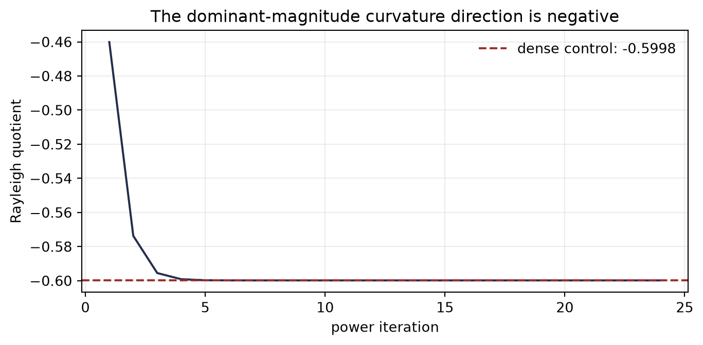
The opening model is only two-dimensional, so we can use its dense Hessian as a control while the iteration sees only an action function.

1. Reuse the verified composed-logit witness.
2. Define a function that accepts a vector and returns \(\matr{H}\vect{v}\).
3. Check one action against dense multiplication.
4. Run seeded power iteration through the action interface.
5. Compare the signed estimate with the dense eigendecomposition.
6. Verify the second committed claim artifact.

from trainable_harness import (
    bernoulli_hessian_vector_product,
    dominant_symmetric_eigenpair,
)

# [1]
assert manifest["harness_ref"] == "ch-12"

# [2]
def hessian_action(vector):
    return bernoulli_hessian_vector_product(
        parameters,
        inputs,
        labels,
        vector,
        nonlinear_first_parameter=True,
    )

# [3]
probe = np.array([0.3, -0.7])
dense_product = composed.hessian @ probe
operator_product = hessian_action(probe)
assert np.allclose(dense_product, operator_product, atol=1e-12, rtol=0.0)

# [4]
estimate = dominant_symmetric_eigenpair(
    hessian_action,
    dimension=2,
    iterations=24,
    seed=6212,
)

# [5]
dense_eigenvalues = np.linalg.eigvalsh(composed.hessian)
dominant = dense_eigenvalues[np.argmax(np.abs(dense_eigenvalues))]
assert np.isclose(estimate.eigenvalue, dominant, atol=1e-8, rtol=0.0)
iterations = np.arange(1, len(estimate.rayleigh_trace) + 1)
fig, axis = plt.subplots(figsize=(7.2, 3.6))
axis.plot(iterations, estimate.rayleigh_trace, color="#232D4B")
axis.axhline(
    dominant,
    color="#9C2F2F",
    linestyle="--",
    label=f"dense control: {dominant:.4f}",
)
axis.set(
    xlabel="power iteration",
    ylabel="Rayleigh quotient",
    title="The dominant-magnitude curvature direction is negative",
)
axis.grid(alpha=0.22)
axis.legend(frameon=False)
fig.tight_layout()

# [6]
hvp_claim = verify_claim("c12-hvp-001", expected_harness=pin)
assert np.allclose(
    hvp_claim["result"]["operator_product"],
    operator_product,
    atol=1e-12,
    rtol=0.0,
)
assert np.isclose(
    hvp_claim["result"]["dominant_magnitude_eigenvalue_estimate"],
    estimate.eigenvalue,
    atol=1e-12,
    rtol=0.0,
)
print(
    "claim c12-hvp-001: verified; "
    f"eigenvalue={estimate.eigenvalue:.10f}; "
    f"residual={estimate.residual_norm:.3e}"
)

claim c12-hvp-001: verified; eigenvalue=-0.5998303709; residual=2.807e-10

Figure 12.2: Matrix-free power iteration approaches the Hessian eigenvalue of largest magnitude. The estimate is negative because magnitude, not algebraic order, governs ordinary power iteration.

WarningNamed wrong answer: power iteration finds the largest eigenvalue

Ordinary power iteration targets the eigenvalue of largest magnitude when one is uniquely dominant. It does not automatically target the largest algebraic eigenvalue. Here that distinction is the difference between reporting negative curvature and erasing it.

The point of the operator interface is larger than this tiny witness. Lanczos iteration, conjugate gradients, trace estimators, and several second-order diagnostics can be written in terms of matrix–vector products. The matrix is then defined by what action the program computes. That makes the choice among \(\matr{H}\), \(\matr{G}\), \(\matr{F}\), and \(\widetilde{\matr{F}}\) an executable API decision.

12.5 Object, representation, and solver are separate choices

Three decisions are often compressed into the phrase “use second order”:

Decision	Examples	Question it answers
curvature object	\(\matr{H}\), \(\matr{G}\), \(\matr{F}\), \(\widetilde{\matr{F}}\)	What local geometry is being represented?
representation	exact action, diagonal, blocks, low rank, structured factorization	What information is retained and affordable?
solver or use	power iteration, conjugate gradients, damping, preconditioning	What action is taken with that representation?

A diagonal Hessian and a diagonal Fisher differ before either becomes diagonal. A low-rank approximation can be applied to an indefinite Hessian or a positive-semidefinite GGN. Damping changes the system being solved; it does not retroactively make an empirical Fisher into a model Fisher.

This separation is also a hardware boundary. A matrix-free action avoids storing \(p^2\) entries, but it can still reread activations, replay derivative graphs, and perform reductions. “Matrix free” is a storage statement until a measurement establishes more. CPU timing here would not establish accelerator performance.

Representation can also change the numerical problem before a solver takes a step. Let \(\matr{J}\in\mathbb{R}^{m\times p}\) have full column rank, with singular values \(\sigma_1\ge\cdots\ge\sigma_p>0\). The eigenvalues of \(\matr{J}^{\mathsf T}\matr{J}\) are \(\sigma_i^2\), so

\[ \kappa_2(\matr{J}^{\mathsf T}\matr{J}) = \frac{\sigma_1^2}{\sigma_p^2} = \kappa_2(\matr{J})^2. \tag{12.10}\]

Forming normal equations therefore squares the spectral condition number and can spend roughly twice the digits that the original least-squares operator made vulnerable. This is the C03 precision contract applied to a curvature representation, not a reason to declare one solver universally superior. QR avoids explicitly squaring the operator; LSQR uses products with \(\matr{J}\) and \(\matr{J}^{\mathsf T}\); matrix-free curvature products avoid forming the dense Gram matrix. Each alternative still owes a cost, stopping, precision, and residual contract. Damping replaces the system by a different one rather than undoing the squaring (Higham 2002).

12.6 One linear solver, two lenses

Suppose a positive-definite curvature operator \(\matr{A}\) defines the system \(\matr{A}\vect{x}=\vect{b}\). Conjugate gradients can be read dynamically as a sequence of mutually \(\matr{A}\)-conjugate search directions. It can also be read inferentially: under a Gaussian prior and exact linear observations, the same algebra updates a distribution over the unknown solution (Hennig 2015). These are two interpretations of one computation, not evidence that every iterative solver is Bayesian.

The seam matters because curvature estimation is itself an information problem. Secant pairs reveal actions of an unknown Hessian. Probabilistic quasi-Newton work asks what posterior over a matrix is compatible with those observations (Hennig and Kiefel 2013). This chapter keeps that as a branch from the trunk: students need the operator/observation distinction to read such work, but not the full probabilistic-numerics apparatus to diagnose the opening failure.

TipField note: a curvature card

Before accepting a curvature claim, record five fields: the mathematical object; every averaging distribution; the representation or approximation; the matrix action actually implemented; and the solver, damping, or preconditioning policy that consumes it.

NoteCheck yourself

For an affine logit with Bernoulli negative log likelihood, which term in Equation 12.5 vanishes? Does that equality make the empirical Fisher equal to the model Fisher for an arbitrary observed label? If a power iteration returns a negative Rayleigh quotient, what ordering of eigenvalues must you check before declaring the implementation wrong?

12.7 Okay, so —

• Inherited: reverse accumulation supplies derivative programs, while Act I supplies the language for spectra and operator probes.
• Changed: “the curvature” became a declared object with an averaging distribution, representation, and consumer.
• Instrumented: the same loss and data produced an indefinite Hessian, a positive-semidefinite GGN/model Fisher, and a different empirical Fisher; an action-only power iteration recovered the signed dominant-magnitude mode.
• Established: the Hessian splits into GGN plus model curvature; the Fisher identity requires a model expectation and regularity; dense Hessians are unnecessary when the diagnostic needs only \(\matr{H}\vect{v}\); forming \(\matr{J}^{\mathsf T}\matr{J}\) squares \(\matr{J}\)’s spectral condition number when \(\matr{J}\) has full column rank.
• Unresolved: Even with the curvature object named, when does a stochastic gradient estimator predict descent rather than noise-dominated motion?

12.8 Sources and further reading

The matrix-free Hessian–vector identity and its implementation boundaries follow Pearlmutter (1994). The distinctions among the Hessian, generalized Gauss–Newton matrix, Fisher information, and empirical Fisher are checked against Martens (2020) and Kunstner et al. (2019). The inferential interpretation of conjugate gradients follows Hennig (2015); the quasi-Newton branch follows Hennig and Kiefel (2013). The normal-equations precision boundary follows the singular-value calculation on the page and the numerical linear algebra contract in Higham (2002). The ICML probabilistic-numerics tutorial supplied an intellectual seam, not the technical authority for these claims.

Reading order. Start with Martens (2020) and Kunstner et al. (2019) to name the curvature object, use Pearlmutter (1994) for action-only computation, and then read Hennig (2015) or Hennig and Kiefel (2013) for the bounded inferential branches.

12.9 Exercises

1. (Pencil.) Starting from Equation 12.1, derive all four numbers in Equation 12.2. Then replace \(y=1\) with \(y=0\) without changing \(w\). Which quantities change, and which remain fixed?
2. (Pencil.) Give a scalar example in which the model-curvature term \(\matr{R}\) in Equation 12.5 is positive. Explain why this disproves the claim that GGN merely deletes negative Hessian curvature.
3. (Code.) Replace the two-parameter witness by a small nonlinear model. Implement Hessian and GGN actions, then use the same Lanczos or power iteration driver on both. Report the signed extremal Ritz values and an operator-residual check.
4. (Code.) For Bernoulli logits, simulate labels from the current model and average observed-label score outer products. Show convergence toward the model Fisher, then repeat with labels from a misspecified distribution.
5. (Audit.) Paper audit: Select a paper that reports a Fisher, GGN, or Hessian spectrum. Complete the Mathematical object, Estimator and comparison contract, Evidence culture and interface, Assumption stress test, and Transfer verdict fields. Identify the expectation implemented by the code, whether the reported matrix is exact or approximated, and which conclusion would fail if the object were replaced by the empirical Fisher.

Hennig, Philipp. 2015. “Probabilistic Interpretation of Linear Solvers.” SIAM Journal on Optimization 25 (1): 234–60. https://doi.org/10.1137/140955501.

Hennig, Philipp, and Martin Kiefel. 2013. “Quasi-Newton Methods: A New Direction.” Journal of Machine Learning Research 14: 843–65. https://www.jmlr.org/papers/v14/hennig13a.html.

Higham, Nicholas J. 2002. Accuracy and Stability of Numerical Algorithms. 2nd ed. Society for Industrial; Applied Mathematics. https://doi.org/10.1137/1.9780898718027.

Kunstner, Frederik, Lukas Balles, and Philipp Hennig. 2019. “Limitations of the Empirical Fisher Approximation for Natural Gradient Descent.” Advances in Neural Information Processing Systems 32. https://proceedings.neurips.cc/paper/2019/hash/46a558d97954d0692411c861cf78ef79-Abstract.html.

Martens, James. 2020. “New Insights and Perspectives on the Natural Gradient Method.” Journal of Machine Learning Research 21 (146): 1–76. https://www.jmlr.org/papers/v21/17-678.html.

Pearlmutter, Barak A. 1994. “Fast Exact Multiplication by the Hessian.” Neural Computation 6 (1): 147–60. https://doi.org/10.1162/neco.1994.6.1.147.