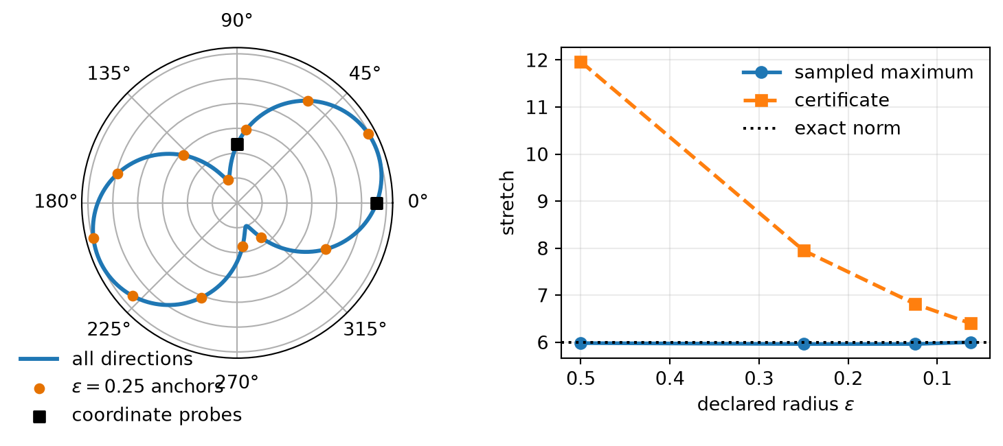
Consider a linear map \(\matr{A}:\mathbb{R}^2\to\mathbb{R}^2\) with singular values \(6\) and \(1\). Rotate its most stretched direction away from both coordinate axes. The largest stretch seen by those two predeclared probes is about \(5.606\). The true maximum is \(6\).
Nothing random or numerically unstable happened. The probes answered the questions they were asked. The direction that maximizes \(\norm{\matr{A}\vect{x}}_2\) is selected after\(\matr{A}\) is known, whereas the coordinate probes were selected before it.
ImportantPrediction
Suppose a probability bound controls each one of one million predeclared directions. Does it control every direction on the unit sphere? If not, name the additional deterministic fact that would let the finite calculation reach the continuum.
7.1 A sampled maximum is not a supremum
C05 paid a logarithmic price for finitely many random variables. C06 showed that the price depends on the tail class. Neither chapter authorized a union bound over an uncountable sphere.
The opening study makes the missing step inspectable. An epsilon-net is a finite set of anchors close enough to every point in the target set. The largest anchor value can still underestimate the true maximum. The covering radius supplies a deterministic correction that turns the underestimate into an upper certificate.
Load the chapter-pinned covering instruments.
Construct a rotated map with known singular values.
Evaluate its stretch over the entire circle and on verified epsilon-nets.
Compute the sampled maximum and interpolation certificate separately.
Plot the hidden direction, anchors, and certificate gap.
Figure 7.1: A finite cover converts missed extrema into a certificate. At left, the stretch of a rotated map varies over the unit circle; the coordinate probes miss the peak, and a verified one-quarter net samples it closely. At right, finer nets close the sampled gap while the deterministic one-over-one-minus-epsilon certificate remains above the exact operator norm. The sampled maximum and the certificate are different quantities.
The net with declared radius \(0.25\) uses \(13\) points. Its sampled maximum is about \(5.963\), still below \(6\). The theorem below turns that shortfall into a valid statement: \(5.963/(1-0.25)\approx7.950\) is conservative, but it cannot miss the true norm.
This is the book’s recurring distinction in geometric form:
Quantity
Meaning
sampled maximum
largest value at the anchors actually evaluated
covering radius
largest permitted distance from any target point to an anchor
interpolation rule
deterministic control of change between nearby points
certificate
sampled maximum plus the declared interpolation cost
true supremum
control value for a small study; usually unavailable at scale
7.2 Make the continuum finite
Let \((K,d)\) be a metric space. A finite subset \(\mathcal{N}_{\epsilon}\subseteq K\) is an epsilon-net of \(K\) when every \(x\in K\) has an anchor \(y\in\mathcal{N}_{\epsilon}\) satisfying \(d(x,y)\le\epsilon\). The covering number
\[
N(K,d,\epsilon)
:=
\min\left\{
|\mathcal{N}|:
\mathcal{N}\text{ is an epsilon-net of }K
\right\}
\tag{7.1}\]
measures the smallest such price. Its logarithm is called the metric entropy.
The word finite matters. In \(\mathbb{R}^d\), a closed and bounded set is compact, so every open cover has a finite subcover. Outside finite-dimensional Euclidean space, boundedness alone does not establish compactness.
Theorem 7.1 (Volumetric upper bound) For every \(\epsilon>0\), the Euclidean unit ball \(B_2^d\) has an epsilon-net with
The same upper bound holds for the unit sphere \(S^{d-1}\).
Proof
Choose a maximal epsilon-separated subset \(\{x_1,\ldots,x_M\}\) of the ball: distinct centers are more than epsilon apart, and no new point can be added while preserving that property. The closed balls of radius \(\epsilon/2\) centered at the \(x_i\) have disjoint interiors. Every one lies inside \((1+\epsilon/2)B_2^d\). Comparing volumes gives
Euclidean volume scales as the \(d\)th power of the radius, hence
\[
M
\le
\left(\frac{1+\epsilon/2}{\epsilon/2}\right)^d
=
\left(1+\frac{2}{\epsilon}\right)^d.
\]
Maximal separation also implies covering: if some point were farther than epsilon from every center, it could be added. The identical packing argument with centers restricted to the sphere proves the sphere upper bound. \(\square\)
The count is exponential in \(d\), but probability calculations pay its logarithm:
This is an upper certificate, not an exact count. For diagnostics, the important question is whether the available tail exponent can pay Equation 7.3.
7.3 Fill the gaps deterministically
A cover controls distances. It does not, by itself, control the function being evaluated. The opening map works because linearity and the operator norm bound the change between nearby directions.
Theorem 7.2 (Operator norm from an epsilon-net) Let \(\mathcal{N}_{\epsilon}\) be an epsilon-net of \(S^{d-1}\) with \(0<\epsilon<1\). For every real matrix \(\matr{A}\) with \(d\) input columns,
Move the last term to the left and divide by \(1-\epsilon\). \(\square\)
WarningNamed wrong answer: ‘Enough random probes make a net’
A cloud of random directions may have good coverage, but sample count alone does not certify its covering radius. The diagnostic needs either a verified construction or a separate probability statement for the random cover. A large probe count is not a geometric certificate.
7.4 Tail budget plus interpolation
The same pattern applies beyond linear maps. Fix a random function \(f_\omega:K\to\mathbb{R}\). The randomness is in \(\omega\); the index \(x\in K\) identifies the query.
Theorem 7.3 (Finite-cover uniformization) Let \(\mathcal{N}_{\epsilon}\) be a finite epsilon-net of \((K,d)\). Suppose every sample path is \(L\)-Lipschitz:
\[
|f_\omega(x)-f_\omega(y)|
\le
L\,d(x,y)
\quad\text{for all }x,y\in K,
\]
and every fixed anchor satisfies the common upper-tail bound
Choose \(t\) so the right side equals \(\delta\). On the complementary event, each \(x\in K\) has an anchor \(y\) within epsilon, and Lipschitz continuity gives
price a cover in the same metric used by the function;
justify the interpolation constant.
If \(L\) is random, the theorem does not permit silently replacing it with its mean. One must first control an event on which \(L\) is bounded, then include that event’s failure probability in the budget.
7.5 Which tails can afford the sphere?
Set \(\epsilon=0.25\) and \(\delta=0.01\). The volumetric upper bound has
\[
\log|\mathcal{N}_{\epsilon}|
\le
d\log 9.
\]
Under a unit-scale sub-Gaussian anchor tail, the union threshold is
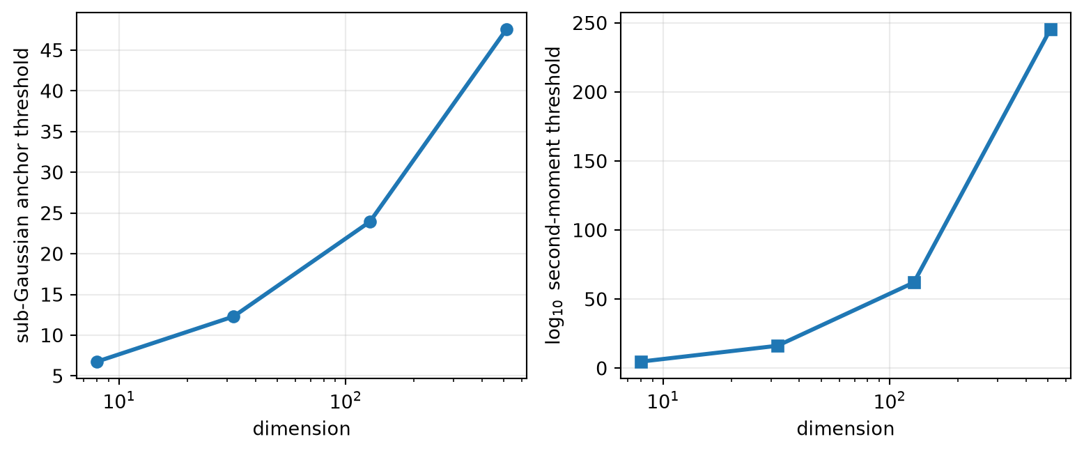
which grows like \(\sqrt d\). Under only the second-moment envelope \(\Pr(|X|\ge t)\le1/t^2\), the same union calculation requires \(t\ge\sqrt{|\mathcal{N}_{\epsilon}|/\delta}\), exponential in \(d\).
The latter calculation is valid. It is simply too weak to give a useful high-dimensional diagnostic.
Fix the covering radius and failure probability.
Compute the log covering upper bound without materializing the cover.
Solve the sub-Gaussian union budget for its threshold.
Solve the second-moment union budget on a log-ten scale.
Figure 7.2: Tail class determines whether an exponential cover is affordable. At left, the sub-Gaussian union threshold grows on a square-root-dimensional scale. At right, the base-ten logarithm of the second-moment threshold grows linearly with dimension; by dimension 512 the threshold is above ten to the 245. Both are valid union calculations under their stated envelopes, but only one is diagnostically useful.
The comparison also explains why C06 had to distinguish tail regimes before this chapter. A linear Bernstein exponent can still pay a finite cover, but its threshold scales like the log covering number rather than its square root. The geometry has not changed; the available probabilistic currency has.
NoteField note: discretization is not quantization
A numerical format supplies representable scalar levels, rounding rules, range limits, and arithmetic semantics. An epsilon-net supplies metric coverage of a declared set. Counting \(2^b\) scalar levels does not establish coverage of a \(d\)-dimensional parameter sphere, and the nearest representable vector need not lie on that sphere. Use C03’s format contract for arithmetic and this chapter’s covering contract for geometry.
The same warning applies to data. A concentration theorem for a declared random model does not prove that a finite training set represents every population the system may encounter. The index set, metric, fixed-point tail, and interpolation rule must all be named.
TipCheck yourself
An epsilon-net has \(N\) anchors. Each fixed anchor obeys \(\Pr(f(y)>a+t)\le2e^{-t^2/(2\sigma^2)}\), and every sample path is \(L\)-Lipschitz. What is the smallest union-bound threshold that gives failure probability delta? Which term changes if the cover is refined from epsilon to epsilon over two, and which term does not?
7.6 Okay, so —
Inherited: C05 supplied fixed-point sub-Gaussian control; C06 turned a tail exponent into a finite statistical budget.
Changed: the target is now a continuum, so probability at anchors is insufficient without geometric coverage and deterministic interpolation.
Instrumented: the harness constructs verified circle nets, measures their actual covering radii, certifies operator norms, and prices sphere covers without materializing them.
Established: Euclidean covers have exponential size but linear log cost; an epsilon-net and a Lipschitz rule convert anchor control into a uniform bound.
Unresolved: How can a finite-cover certificate control extremal singular directions selected only after a random matrix is observed?
7.7 Sources and further reading
Vershynin develops covering and packing numbers, the volumetric upper bound, and epsilon-net arguments for random operators (Vershynin 2026). Baraniuk, Davenport, DeVore, and Wakin combine fixed-vector concentration with finite-dimensional covering numbers in a restricted-isometry proof (Baraniuk et al. 2008).
For the general theory, use Vershynin (2026); this chapter’s contribution is the sampled-maximum versus uniform-certificate diagnostic.
Reading order. Start with Vershynin (2026) for covering numbers and the interpolation lemma, then read Baraniuk et al. (2008) as a complete worked example of a finite tail budget paying for a continuous guarantee.
7.8 Exercises
(Pencil.) A circle cover. Derive the exact chord covering radius of \(k\) equally spaced points on \(S^1\). Find the smallest \(k\) that certifies radius at most \(0.1\), and compare it with the volumetric upper bound.
(Pencil.) Symmetric quadratic forms. Let \(\matr{B}\) be symmetric and \(\mathcal{N}_{\epsilon}\) an epsilon-net of the unit sphere with \(\epsilon<1/2\). Prove \[
\norm{\matr{B}}_{\mathrm{op}}
\le
\frac{1}{1-2\epsilon}
\max_{\vect{x}\in\mathcal{N}_{\epsilon}}
|\vect{x}^{\mathsf T}\matr{B}\vect{x}|.
\] Mark the two interpolation errors that create \(2\epsilon\).
(Code.) Random probes versus a verified cover. In two dimensions, compare \(k\) uniformly random directions with \(k\) equally spaced directions over 10,000 independent probe sets. Report the distribution of the actual covering radius, not only the largest observed stretch.
(Code.) Choose epsilon. For Equation 7.5 with the volumetric sphere bound, minimize the sum of anchor threshold and \(L\epsilon\) numerically over epsilon for several values of \(d\), \(L\), and delta. Explain why the finest cover need not give the smallest final certificate.
(Audit.) A missing regularity contract. A report evaluates a random function at one million directions, applies a union bound, and calls the result a bound on the sphere. Write the strongest claim the evidence actually supports. Then list two distinct regularity statements that could repair the continuum step.
(Audit.) Paper audit: where the cover enters. Complete the Mathematical object, Evidence culture and interface, Assumption stress test, and Discriminating control fields for Baraniuk, Davenport, DeVore, and Wakin (Baraniuk et al. 2008). Identify the fixed-vector concentration statement, the set being covered, the covering-number cost, and the deterministic step extending anchor control. Separate those ingredients from the paper’s additional union over supports.
Baraniuk, Richard, Mark Davenport, Ronald DeVore, and Michael Wakin. 2008. “A Simple Proof of the Restricted Isometry Property for Random Matrices.”Constructive Approximation 28 (3): 253–63. https://doi.org/10.1007/s00365-007-9003-x.
Vershynin, Roman. 2026. High-Dimensional Probability: An Introduction with Applications in Data Science. 2nd ed. Cambridge Series in Statistical and Probabilistic Mathematics. Cambridge University Press. https://www.math.uci.edu/~rvershyn/papers/HDP-book/HDP-book.html.