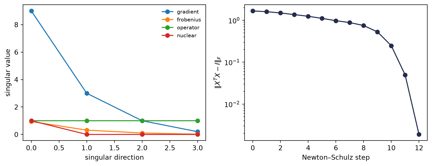
Let a \(6\times4\) gradient matrix have singular values \((9,3,1,0.2)\). Three unit-size update problems return three different answers. A Frobenius-unit step follows the normalized gradient. A nuclear-unit step spends its entire budget on the leading singular pair. An operator-unit step uses the polar factor and gives all four singular directions unit magnitude. Their inner products with the gradient are respectively \(-9.54\), \(-9\), and \(-13.2\).
“Steepest” was never a property of the gradient alone; it was a property of a normed geometry.
ImportantPrediction
A paper replaces a coordinate-wise update by a matrix transformation. Before asking whether it wins, ask: steepest under which norm, for which parameter blocks, with what approximation error, scaling rule, state traffic, and evidence regime?
17.1 One linearization, three unit balls
For a small update \(\matr D\), the first-order change is \(\langle\matr G,\matr D\rangle_F\). Choosing a step means minimizing this linear functional over a declared unit ball.
Theorem 17.1 (Matrix-norm steepest directions) Let \(\matr G=\matr U\operatorname{diag}(\vect\sigma)\matr V^{\mathsf T}\). Then
The Frobenius row is Cauchy–Schwarz. The other rows are duality between the operator and nuclear norms, with equality at the displayed SVD-aligned matrices. Notice the reversal: an operator-norm constraint yields the polar factor; a nuclear-norm constraint yields a rank-one direction.
This is the de-branded trunk beneath recent matrix-aware optimizers. It also returns to C08: singular values of the update are not singular values of the weights, Hessian, or data matrix. Every spectral plot must name its matrix.
Load the chapter-pinned matrix-update instruments.
Construct the registered rectangular gradient.
Compute the three norm-steepest directions.
Approximate the polar factor by Newton–Schulz iteration.
Verify the singular values, inner products, and residual trace.
Figure 17.1: The norm changes the update spectrum. The operator-ball solution replaces every nonzero gradient singular value by one; a short polynomial iteration approaches that polar factor without an SVD.
acts on each singular value as \(s\mapsto 1.5s-0.5s^3\). For \(0<s<\sqrt3\), repeated steps move toward one; zero singular values remain zero. A finite iteration therefore needs a scaling rule, step count, residual metric, dtype, and rank-deficiency policy. In narrow arithmetic, forming the Gram factor and repeated matrix products also reopens C03’s accumulation contract.
The exact polar factor is equivariant: \(\operatorname{polar}(\matr Q\matr G\matr R)=
\matr Q\operatorname{polar}(\matr G)\matr R\) for orthogonal \(\matr Q,\matr R\), and it is invariant to positive scalar rescaling. Those properties explain what coordinate transformations the update respects.
17.3 The update spectrum is not the weight spectrum
The opening compares candidate updates at one gradient. The promise from C08 is stronger: show the update spectrum and the weight spectrum side by side while a model changes. Use a factorized least-squares control
with matched initialization and twenty steps. One run normalizes each factor gradient in Frobenius norm. The other replaces it by the rectangular polar factor. Both then restore an external step scale \(alpha=0.08\).
Derive the claim seed and construct one target and matched factorization.
Run twenty Frobenius-normalized and polar steps.
Record the singular values of each update to factor A.
Record the singular values of factor A before each update.
Plot both spectra over time and verify the committed endpoints.
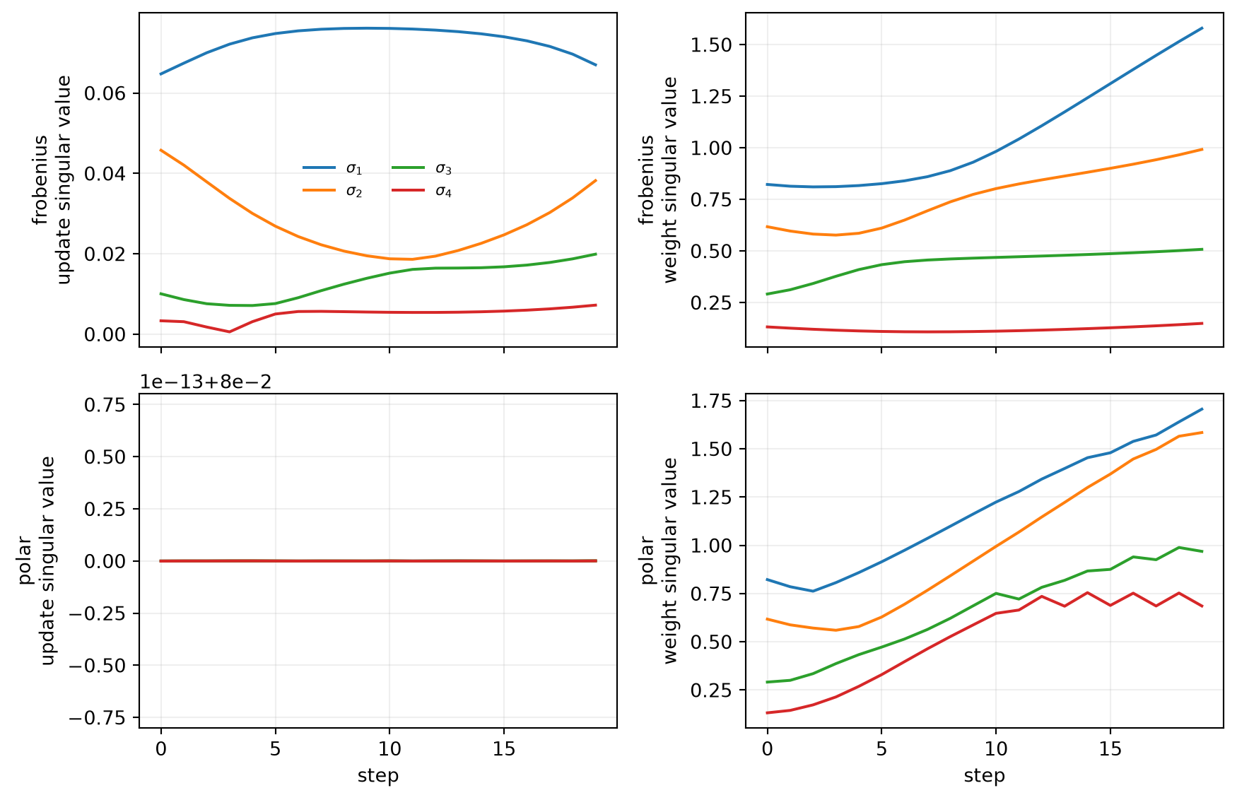
polar update spread: 1.39e-16
polar final weight spectrum: 1.706/1.584/0.969/0.686
Figure 17.2: Update and weight spectra are different objects. Polar steps give all four update singular directions the external scale 0.08 at every iteration, while the factor being updated remains anisotropic and evolves. Frobenius-normalized updates retain unequal singular values.
The polar update is an isometry on the four-dimensional input space at every step: its four singular values are all \(0.08\) up to rounding. Factor \(\matr A\) is not. Its final singular values are approximately \((1.706,1.584,0.969,0.686)\). “Orthogonalized update” therefore describes the step matrix, not the parameter matrix after the step and not the represented function \(\matr A\matr B\).
The control also makes routing and scale explicit:
Parameter block
Routed transformation
Where magnitude re-enters
Audit boundary
matrix factor \(\matr A\)
Frobenius or polar direction
external \(alpha=0.08\)
width and layer scaling omitted
matrix factor \(\matr B\)
same declared rule
external \(alpha=0.08\)
square and rectangular blocks share no automatic scale law
a hypothetical bias vector
excluded
requires a separate vector rule
cannot be silently reshaped into a matrix
This is not an implementation footnote. A method that transforms selected matrices but routes embeddings, biases, scales, or output heads differently is a family of update rules. The paper autopsy must identify all of them.
17.4 One complete matrix-block step
For one matrix block \(\matr W\in\mathbb R^{m\times n}\) with \(m\ge n\), a complete routed step needs more than the polar idealization. Let
Here \(T\) polynomial iterations approximate the polar factor and \(s_{m,n}\) restores a declared external scale. The following kernel exposes the whole block transition:
For FP32 storage, \(\matr W\) and persistent momentum already require \(8mn\) bytes together. One Newton–Schulz step for a tall block forms an \(n\times n\) Gram matrix and performs matrix products costing \(O(mn^2)\) arithmetic. A materialized implementation also moves the block, momentum, iterates, and Gram temporary; fusion or tiling can change that traffic without changing Equation 17.4.
Contract field
This block step declares
Still requires measurement
normalization
Frobenius scale before iteration
overflow/underflow and low-precision accumulation
approximation
\(T\) steps and \(\|X_T^{\mathsf T}X_T-I\|_{\mathrm F}\)
error relative to the exact polar factor
persistent state
one \(m\times n\) momentum matrix
optimizer state for excluded parameters
arithmetic
\(O(Tmn^2)\) for \(m\ge n\)
achieved kernel rate
traffic
at least weights, gradients, momentum, and outputs
cache reuse, fusion, and communication
routing
this matrix block only
biases, scales, embeddings, and output blocks
The table is the algorithmic lens on the same update whose singular values supplied the geometric lens. A paper must own both.
17.5 Brand bridge
Muon applies momentum and then an approximate polar transformation to selected two-dimensional hidden-weight blocks (Jordan 2024; Liu et al. 2025). A useful shorthand is “sign descent on singular values,” but it is a geometric surrogate, not a complete anatomy theorem: parameter routing, external scale, momentum, polynomial coefficients, dtype, and excluded parameters remain part of the method. Published compute-efficiency numbers are paper evidence tied to their hardware and baselines; this chapter does not reproduce them.
QJL (Zandieh et al. 2024) and TurboQuant (Zandieh et al. 2025) belong beside this discussion as a paper-audit branch about communication, quantization, and random projections—not as a second method tutorial. Their claims should be routed through C01’s traffic boundary, C03’s quantizer contract, and C07’s uniformization question.
WarningNamed wrong answer: orthogonalized updates are scale free
The polar map removes positive scalar magnitude from a full-rank matrix. A practical optimizer restores scale elsewhere and carries momentum and state. Audit the entire update, not one transformation.
17.6 The terminal capability: autopsy before adoption
The numbered core closes with a procedure rather than a winner. The Coda then uses the same discipline on a training incident. For a current paper, write a one-page autopsy:
Claim: What is proved, measured, interpreted, or merely proposed?
Mathematical object: Which matrix, estimator, norm, and population or sample quantity is named?
Resolution of the theory: Is the statement global, local, direction-aware, or finite-horizon?
Dynamic regime: Are the argument and experiments gradient- or noise-dominated, light- or heavy-tailed, fixed- or moving-curvature?
Evidence culture and interface: Which measured quantity corresponds to which assumption or conclusion?
Estimator and comparison contract: What are the target, reduction, denominator, sampling scheme, seeds, and baseline budget?
Numerical and hardware contract: Which dtype, scaling, state, bytes, device, and wall-clock protocol carry the endpoint?
Assumption stress test: Which conclusion survives when the most fragile assumption is changed?
Discriminating control: Which smallest control separates the proposed mechanism from its strongest rival?
Transfer verdict: State what is supported, what is not, and the cheapest next test.
This combines the course’s Spring 2026 optimizer card with the theory-resolution and two-cultures maps. Credit the tutorial for its intellectual map and the primary paper for technical claims. Do not attribute the combined checklist to either source.
17.7 Check yourself
For singular values \((9,3,1,0.2)\), what are the operator-ball and nuclear-ball minimum values, and which dual norms produce them? If a Newton–Schulz approximation has residual \(10^{-3}\), which claim does that support, and which two tempting optimizer claims remain unsupported?
Changed: an optimizer is read as a normed update contract plus approximation, routing, state, and evidence.
Instrumented: one claim compares three dual geometries and a polynomial approximation; another separates update spectra from evolving weight spectra.
Established: the norm chooses the steepest direction; the method name does not.
Unresolved: When one loss spike activates several instruments, which control identifies the cause rather than merely detecting the event?
17.9 Sources and further reading
Matrix-norm steepest descent and recent optimizer connections are developed by Bernstein and Newhouse (2024). The original Muon technical account is Jordan (2024), with large-scale implementation evidence in Liu et al. (2025). The neighboring matrix-preconditioning artifacts are Shampoo (Gupta et al. 2018) and SOAP (Vyas et al. 2024). For the diagonal-moment and decoupled-decay baselines, see Kingma and Ba (2015) and Loshchilov and Hutter (2019). The quantized-projection audit branch starts with Zandieh et al. (2024) and continues with Zandieh et al. (2025).
Reading order. Start with Bernstein and Newhouse (2024) for dual-norm geometry, then audit Jordan (2024) and Liu et al. (2025) in that order: mathematical update contract first, scaling evidence second. If quantization is the target, read Zandieh et al. (2024) before Zandieh et al. (2025).
17.10 Exercises
(Pencil.) Prove the operator/nuclear duality rows of Equation 17.1 using von Neumann’s trace inequality.
(Code.) Test Newton–Schulz across condition numbers, ranks, and dtypes. Separate polar error, orthogonality residual, and elapsed time.
(Pencil.) For the factorized control, derive both factor gradients and show why an isometric update to each factor does not imply an isometric update to their product.
(Code.) Add vector biases and per-layer scale factors to the trace. Implement an explicit routing table and, under equal nominal learning rates, compare update spectra, weight spectra, state bytes, final loss, and each block’s induced output change or Jacobian-Gram contribution. Explain why equal parameter-step norms need not produce equal function-space steps.
(Audit.) Paper audit: Apply all ten fields of the Paper Autopsy Protocol to one routed matrix-update, quantization, or edge-of-stability paper. For the quantization branch, begin with Zandieh et al. (2024) or Zandieh et al. (2025) rather than a method name alone. End by naming the single assumption whose failure would most weaken its central claim.
(Audit.) Act checkpoint — complete Incident Card. For a run rather than a paper, keep this fixed order: Symptom → Prediction → Contract → Precision control → Curvature control → Estimator control → Spectrum locator → State control → Verdict → Corrective control. Complete the Act II assignment. Route: Act checkpoint. Estimated time: 90 minutes. Deliverable: one complete card plus the cheapest discriminating rerun. Hint: an activated instrument may detect the event without identifying its cause.
Gupta, Vineet, Tomer Koren, and Yoram Singer. 2018. “Shampoo: Preconditioned Stochastic Tensor Optimization.”Proceedings of the 35th International Conference on Machine Learning, Proceedings of machine learning research, vol. 80: 1842–50. https://proceedings.mlr.press/v80/gupta18a.html.
Kingma, Diederik P., and Jimmy Ba. 2015. “Adam: A Method for Stochastic Optimization.”International Conference on Learning Representations. https://doi.org/10.48550/arXiv.1412.6980.
Loshchilov, Ilya, and Frank Hutter. 2019. “Decoupled Weight Decay Regularization.”International Conference on Learning Representations. https://doi.org/10.48550/arXiv.1711.05101.